---
title: "What Is Driving NDIS Spend Growth?"
description: "A reproducible first pass at explaining NDIS spend growth using public participant, payment, budget, utilisation and regional data."
date: "2026-05-26"
categories: [ndis, health-policy, modelling, australia]
author: "Aydin"
---
The National Disability Insurance Scheme is usually discussed through one big number: total spend. That is not wrong, but it hides several different mechanisms. Spend can grow because more people enter the scheme, because average plan budgets rise, because participants use more of their approved supports, or because the participant mix changes toward groups with higher support needs.
This post uses the short public quarterly window to tell a descriptive spend-growth story:
1. How quickly is observed NDIS spend growing?
2. Is scheme participation growing faster than the Australian population?
3. Is spend pressure coming more from participant growth, average budgets, or utilisation?
4. Which disability groups appear largest, most expensive, and fastest growing?
5. What public explanatory factors help describe grouped quarterly spend?
The models are descriptive, not funding advice and not a participant-level forecast. I deliberately avoid lagged payment and lagged budget features in the overall spend model: those improve fit, but they mostly tell us that last quarter predicts this quarter. The aim here is to describe observable drivers.
```{r}
#| label: setup
#| include: false
library(readr)
library(dplyr)
library(tidyr)
library(ggplot2)
library(stringr)
library(purrr)
library(lubridate)
library(forcats)
library(readxl)
library(broom)
library(scales)
library(knitr)
library(randomForest)
theme_set(theme_minimal(base_size = 12))
raw_dir <- file.path("data-raw", "ndis")
dir.create(raw_dir, recursive = TRUE, showWarnings = FALSE)
analysis_quarters <- tibble::tribble(
~quarter_label, ~quarter_date, ~quarter_index,
"March 2024", "2024-03-31", 1,
"June 2024", "2024-06-30", 2,
"September 2024", "2024-09-30", 3,
"December 2024", "2024-12-31", 4,
"March 2025", "2025-03-31", 5,
"June 2025", "2025-06-30", 6,
"September 2025", "2025-09-30", 7,
"December 2025", "2025-12-31", 8
) |>
mutate(quarter_date = as.Date(quarter_date))
page_urls <- list(
participant = "https://dataresearch.ndis.gov.au/datasets/participant-datasets",
provider = "https://dataresearch.ndis.gov.au/datasets/provider-datasets",
payments = "https://dataresearch.ndis.gov.au/datasets/payments-datasets",
outcomes = "https://dataresearch.ndis.gov.au/reports-and-analyses/outcomes-and-goals/participant-families-and-carer-outcomes-reports",
national_population = "https://www.abs.gov.au/statistics/people/population/national-state-and-territory-population/latest-release",
seifa = "https://www.abs.gov.au/statistics/people/people-and-communities/socio-economic-indexes-areas-seifa-australia/latest-release",
seifa_lga = "https://www.abs.gov.au/statistics/people/people-and-communities/socio-economic-indexes-areas-seifa-australia/2021/Local%20Government%20Area%2C%20Indexes%2C%20SEIFA%202021.xlsx",
population_age_lga = "https://www.abs.gov.au/statistics/people/population/regional-population-age-and-sex/2021/32350DS0004_2021.xlsx",
asgs_mb_2021 = "https://www.abs.gov.au/statistics/standards/australian-statistical-geography-standard-asgs/edition-3-july-2021-june-2026/access-and-downloads/allocation-files/MB_2021_AUST.xlsx",
asgs_lga_2021 = "https://www.abs.gov.au/statistics/standards/australian-statistical-geography-standard-asgs/edition-3-july-2021-june-2026/access-and-downloads/allocation-files/LGA_2021_AUST.xlsx",
asgs_ra_2021 = "https://www.abs.gov.au/statistics/standards/australian-statistical-geography-standard-asgs/edition-3-july-2021-june-2026/access-and-downloads/allocation-files/RA_2021_AUST.xlsx",
population_age = "https://www.abs.gov.au/statistics/people/population/regional-population-age-and-sex/2021"
)
```
## Data Sources
The workflow downloads source files from the [NDIS participant datasets](https://dataresearch.ndis.gov.au/datasets/participant-datasets), [NDIS provider datasets](https://dataresearch.ndis.gov.au/datasets/provider-datasets), and [NDIS payments datasets](https://dataresearch.ndis.gov.au/datasets/payments-datasets). It focuses on plan budgets, utilisation, providers, market concentration, payments, and LGA mapping files. It also uses ABS estimated resident population from [National, state and territory population](https://www.abs.gov.au/statistics/people/population/national-state-and-territory-population/latest-release), then tries to add regional context from [SEIFA 2021](https://www.abs.gov.au/statistics/people/people-and-communities/socio-economic-indexes-areas-seifa-australia/2021) and population age structure. If the ABS files change shape, the NDIS-only analysis still runs and reports the missing context.
```{r}
#| label: helpers
clean_names <- function(x) {
  x |>
    str_to_lower() |>
    str_replace_all("&", "and") |>
    str_replace_all("[^a-z0-9]+", "_") |>
    str_replace_all("^_|_$", "")
}

clean_df <- function(x) {
  names(x) <- clean_names(names(x))
  x
}

as_number <- function(x) {
  if (is.numeric(x)) return(x)
  x_chr <- as.character(x)
  out <- parse_number(x_chr, na = c("", "NA", "n/a", "Not applicable", "No data available"))
  ifelse(str_detect(x_chr, "^\\s*<"), NA_real_, out)
}

as_rate <- function(x) {
  out <- as_number(x)
  ifelse(out > 1.5, out / 100, out)
}

safe_sum <- function(x) {
  x <- x[is.finite(x)]
  if (length(x) == 0) return(NA_real_)
  sum(x)
}

safe_mean <- function(x) {
  x <- x[is.finite(x)]
  if (length(x) == 0) return(NA_real_)
  mean(x)
}

safe_median <- function(x) {
  x <- x[is.finite(x)]
  if (length(x) == 0) return(NA_real_)
  median(x)
}

safe_mode_character <- function(x) {
  x <- as.character(x)
  x <- x[!is.na(x) & x != "" & x != "ALL"]
  if (length(x) == 0) return(NA_character_)
  names(sort(table(x), decreasing = TRUE))[[1]]
}

collapse_top_values <- function(x, n = 4) {
  x <- as.character(x)
  x <- unique(x[!is.na(x) & x != "" & x != "ALL"])
  if (length(x) == 0) return(NA_character_)
  paste(head(sort(x), n), collapse = ", ")
}

safe_weighted_mean <- function(x, w) {
  x <- as.numeric(x)
  w <- as.numeric(w)
  keep <- is.finite(x) & is.finite(w) & w > 0
  if (any(keep)) return(weighted.mean(x[keep], w[keep]))
  safe_mean(x)
}

has_enough_data <- function(data, cols, min_rows = 2) {
  if (nrow(data) < min_rows) return(FALSE)
  all(map_lgl(cols, \(col) col %in% names(data) && sum(is.finite(data[[col]])) >= min_rows))
}

format_optional_number <- function(x, accuracy = 0.1, suffix = "") {
  ifelse(is.na(x) | !is.finite(x), "Not joined", paste0(number(x, accuracy = accuracy), suffix))
}

format_optional_percent <- function(x, accuracy = 0.1) {
  ifelse(is.na(x) | !is.finite(x), "Not joined", percent(x, accuracy = accuracy))
}

index_to_first <- function(x) {
  bases <- x[is.finite(x) & x > 0]
  base <- if (length(bases) > 0) bases[[1]] else NA_real_
  if (length(base) == 0 || is.na(base)) return(rep(NA_real_, length(x)))
  x / base - 1
}

pretty_feature <- function(x) {
  recode(
    x,
    quarter_index = "time",
    log_participants = "participant count",
    log_providers = "active providers",
    log_participants_per_provider = "participants per active provider",
    payment_share_top10 = "top-10 provider payment share",
    irsd_score = "SEIFA disadvantage score",
    irsd_decile = "SEIFA disadvantage decile",
    ier_score = "economic resources score",
    ier_decile = "economic resources decile",
    ieo_score = "education/occupation score",
    ieo_decile = "education/occupation decile",
    median_age = "median local age",
    pct_0_14 = "local population aged 0-14",
    pct_15_64 = "local population aged 15-64",
    pct_65_plus = "local population aged 65+",
    log_lga_population = "local population",
    remoteness_rank = "remoteness",
    remoteness_major_cities_share = "major-cities share",
    remoteness_inner_regional_share = "inner-regional share",
    remoteness_outer_regional_share = "outer-regional share",
    remoteness_remote_share = "remote share",
    remoteness_very_remote_share = "very-remote share",
    log_budget = "average support budget",
    state = "state",
    service_district = "service district",
    age_group = "age group",
    disability_group = "disability group",
    support_class = "support class",
    remoteness = "remoteness",
    .default = str_replace_all(x, "_", " ")
  )
}

top_rf_predictors <- function(model, n = 5) {
  importance(model) |>
    as.data.frame() |>
    tibble::rownames_to_column("feature") |>
    arrange(desc(IncNodePurity)) |>
    slice_head(n = n) |>
    pull(feature) |>
    pretty_feature() |>
    paste(collapse = ", ")
}

first_col <- function(data, patterns, required = TRUE) {
  hits <- names(data)[map_lgl(names(data), \(nm) any(str_detect(nm, regex(paste(patterns, collapse = "|"), ignore_case = TRUE))))]
  if (length(hits) == 0) {
    if (required) stop("Could not find column matching: ", paste(patterns, collapse = ", "))
    return(NA_character_)
  }
  hits[[1]]
}

sample_rows <- function(data, n = 8000) {
  data |> slice_sample(n = min(nrow(data), n))
}

normalise_service_district <- function(x) {
  x |>
    as.character() |>
    str_replace("^[A-Z]{2,3}~", "") |>
    str_squish()
}

read_page <- function(url) {
  paste(readLines(url, warn = FALSE, encoding = "UTF-8"), collapse = "\n")
}

extract_links <- function(url) {
  html <- read_page(url)
  base_url <- str_replace(url, "^(https?://[^/]+).*$", "\\1")
  matches <- gregexpr("<a[^>]+href=[\"']([^\"']+)[\"'][^>]*>(.*?)</a>", html, perl = TRUE)
  pieces <- regmatches(html, matches)[[1]]
  if (length(pieces) == 0) return(tibble(label = character(), url = character()))
  tibble(raw = pieces) |>
    mutate(
      href = str_match(raw, "href=[\"']([^\"']+)[\"']")[, 2],
      label = raw |>
        str_replace_all("<[^>]+>", " ") |>
        str_squish(),
      url = case_when(
        str_detect(href, "^https?://") ~ href,
        str_detect(href, "^/") ~ paste0(base_url, href),
        TRUE ~ paste0(str_remove(url, "/[^/]*$"), "/", href)
      )
    ) |>
    select(label, url)
}

quarter_from_label <- function(label) {
  month <- str_match(label, "(March|June|September|December)")[, 2]
  year <- str_match(label, "(20[0-9]{2})")[, 2]
  tibble(quarter_label = paste(month, year)) |>
    left_join(analysis_quarters, by = "quarter_label")
}

download_one <- function(url, filename) {
  path <- file.path(raw_dir, filename)
  if (!file.exists(path) || (str_detect(filename, "\\.xlsx?$") && !is_xlsx_file(path))) {
    download.file(url, path, mode = "wb", quiet = TRUE)
  }
  path
}

download_quarterly <- function(page_url, label_regex, prefix) {
  links <- extract_links(page_url) |>
    filter(str_detect(label, regex(label_regex, ignore_case = TRUE))) |>
    mutate(row_id = row_number()) |>
    bind_cols(quarter_from_label(extract_links(page_url) |>
      filter(str_detect(label, regex(label_regex, ignore_case = TRUE))) |>
      pull(label))) |>
    select(-row_id) |>
    filter(!is.na(quarter_date), quarter_label %in% analysis_quarters$quarter_label) |>
    distinct(quarter_label, .keep_all = TRUE) |>
    arrange(quarter_date)

  missing <- setdiff(analysis_quarters$quarter_label, links$quarter_label)
  if (length(missing) > 0) {
    message("Missing visible links for ", prefix, ": ", paste(missing, collapse = ", "))
  }

  links |>
    mutate(
      path = map2_chr(url, quarter_label, \(u, q) {
        download_one(u, paste0(prefix, "_", str_replace_all(str_to_lower(q), " ", "_"), ".csv"))
      })
    )
}

is_xlsx_file <- function(path) {
  sig <- readBin(path, what = "raw", n = 4)
  identical(as.integer(sig[1:2]), as.integer(charToRaw("PK")))
}

read_public_table <- function(path) {
  out <- if (is_xlsx_file(path) || str_detect(path, regex("\\.xls$|\\.xlsx$", ignore_case = TRUE))) {
    read_excel(path) |> clean_df()
  } else {
    read_csv(path, show_col_types = FALSE) |> clean_df()
  }
  out |> mutate(across(everything(), as.character))
}

read_quarterly_csvs <- function(links) {
  links |>
    mutate(data = map(path, read_public_table)) |>
    select(quarter_label, quarter_date, quarter_index, data) |>
    unnest(data)
}

download_named <- function(page_url, label_regex, filename) {
  link <- extract_links(page_url) |>
    filter(str_detect(label, regex(label_regex, ignore_case = TRUE))) |>
    slice(1)
  if (nrow(link) == 0) return(NA_character_)
  download_one(link$url[[1]], filename)
}

extension_from_url <- function(url, default = ".csv") {
  ext <- str_match(str_to_lower(url), "\\.(csv|xlsx|xls|zip)(\\?|$)")[, 2]
  ifelse(is.na(ext), default, paste0(".", ext))
}

download_matching <- function(page_url, label_regex, prefix, limit = Inf) {
  links <- extract_links(page_url) |>
    filter(str_detect(label, regex(label_regex, ignore_case = TRUE))) |>
    distinct(label, url) |>
    slice_head(n = limit)

  if (nrow(links) == 0) {
    return(tibble(label = character(), url = character(), path = character()))
  }

  links |>
    mutate(
      path = pmap_chr(list(url, label, row_number()), \(u, lab, i) {
        safe_label <- lab |>
          str_to_lower() |>
          str_replace_all("[^a-z0-9]+", "_") |>
          str_replace_all("^_|_$", "") |>
          str_trunc(70, ellipsis = "")
        download_one(u, paste0(prefix, "_", str_pad(i, 2, pad = "0"), "_", safe_label, extension_from_url(u)))
      })
    )
}
```
```{r}
#| label: download-data
budget_links <- download_quarterly(
  page_urls$participant,
  "^Participant numbers and plan budgets data",
  "participant_plan_budgets"
)

utilisation_links <- download_quarterly(
  page_urls$participant,
  "^Utilisation of Plan budgets data",
  "plan_utilisation"
)

provider_links <- download_quarterly(
  page_urls$provider,
  "^Active providers data",
  "active_providers"
)

budget_raw <- read_quarterly_csvs(budget_links)
utilisation_raw <- read_quarterly_csvs(utilisation_links)
provider_raw <- read_quarterly_csvs(provider_links)

lga_path <- download_named(page_urls$participant, "^Participants by LGA data", "participants_by_lga.csv")
service_lga_path <- download_named(page_urls$participant, "^Service District to LGA 2021 data", "service_district_to_lga_2021.csv")
market_path <- download_named(page_urls$provider, "^Market Concentration data", "market_concentration.csv")
payments_links <- download_quarterly(page_urls$payments, "^Payments data", "payments")
payments_raw <- read_quarterly_csvs(payments_links)

baseline_outcomes_path <- download_named(page_urls$participant, "^Baseline Outcomes data", "baseline_outcomes.csv")
longitudinal_outcomes_path <- download_named(page_urls$participant, "^Longitudinal Outcomes data", "longitudinal_outcomes.csv")
regional_outcome_links <- download_matching(page_urls$outcomes, "by Service District Accessible", "regional_outcomes_service_district")
```
```{r}
#| label: standardise-data
standardise_budget <- function(data) {
  state <- first_col(data, c("^state", "state_territory"), required = FALSE)
  if (is.na(state)) state <- first_col(data, c("state_cd", "statecd"), required = FALSE)
  service <- first_col(data, c("service_district", "srvc_dstrct_nm", "srvcdstrctnm"), required = FALSE)
  age <- first_col(data, c("^age", "age_group", "age_band", "age_bnd", "agebnd"), required = FALSE)
  disability <- first_col(data, c("disability", "dsblty_grp_nm", "dsbltygrpnm"), required = FALSE)
  support <- first_col(data, c("support_class", "support_category", "supp_class", "suppclass", "support"), required = FALSE)
  participants <- first_col(data, c("active.*participant", "actv_prtcpnt", "actvprtcpnt", "number.*participant", "participant.*count", "participants"), required = FALSE)
  budget <- first_col(data, c("average.*support", "average.*budget", "average.*annual", "avg.*annual", "avg_anlsd_cmtd_supp_bdgt", "avganlsdcmtdsuppbdgt", "committed"), required = TRUE)

  data |>
    transmute(
      quarter_label, quarter_date, quarter_index,
      state = if (!is.na(state)) .data[[state]] else NA_character_,
      service_district = if (!is.na(service)) normalise_service_district(.data[[service]]) else NA_character_,
      age_group = if (!is.na(age)) .data[[age]] else NA_character_,
      disability_group = if (!is.na(disability)) .data[[disability]] else NA_character_,
      support_class = if (!is.na(support)) .data[[support]] else NA_character_,
      participant_count = if (!is.na(participants)) as_number(.data[[participants]]) else NA_real_,
      avg_support_budget = as_number(.data[[budget]])
    ) |>
    filter(!is.na(avg_support_budget), state != "ALL", service_district != "ALL", age_group != "ALL", disability_group != "ALL", support_class != "ALL")
}

standardise_national_participants <- function(data) {
  state <- first_col(data, c("^state", "state_territory"), required = FALSE)
  if (is.na(state)) state <- first_col(data, c("state_cd", "statecd"), required = FALSE)
  service <- first_col(data, c("service_district", "srvc_dstrct_nm", "srvcdstrctnm"), required = FALSE)
  age <- first_col(data, c("^age", "age_group", "age_band", "age_bnd", "agebnd"), required = FALSE)
  disability <- first_col(data, c("disability", "dsblty_grp_nm", "dsbltygrpnm"), required = FALSE)
  support <- first_col(data, c("support_class", "support_category", "supp_class", "suppclass", "support"), required = FALSE)
  participants <- first_col(data, c("active.*participant", "actv_prtcpnt", "actvprtcpnt", "number.*participant", "participant.*count", "participants"), required = FALSE)

  if (is.na(participants)) {
    return(tibble(
      quarter_label = character(), quarter_date = as.Date(character()),
      quarter_index = numeric(), ndis_participants = numeric(),
      participant_basis = character()
    ))
  }

  data |>
    transmute(
      quarter_label, quarter_date, quarter_index,
      state = if (!is.na(state)) .data[[state]] else NA_character_,
      service_district = if (!is.na(service)) normalise_service_district(.data[[service]]) else NA_character_,
      age_group = if (!is.na(age)) .data[[age]] else NA_character_,
      disability_group = if (!is.na(disability)) .data[[disability]] else NA_character_,
      support_class = if (!is.na(support)) .data[[support]] else NA_character_,
      participant_count = as_number(.data[[participants]])
    ) |>
    filter(is.finite(participant_count), participant_count > 0) |>
    mutate(
      detail_count = rowSums(across(
        c(state, service_district, age_group, disability_group, support_class),
        \(x) !is.na(x) & x != "ALL"
      ))
    ) |>
    group_by(quarter_label, quarter_date, quarter_index) |>
    filter(detail_count == min(detail_count, na.rm = TRUE)) |>
    summarise(
      ndis_participants = sum(participant_count, na.rm = TRUE),
      detail_count = min(detail_count, na.rm = TRUE),
      participant_basis = if_else(detail_count == 0, "National aggregate row", "Least-detailed rows summed"),
      .groups = "drop"
    )
}

standardise_utilisation <- function(data) {
  state <- first_col(data, c("^state", "state_territory"), required = FALSE)
  if (is.na(state)) state <- first_col(data, c("state_cd", "statecd"), required = FALSE)
  service <- first_col(data, c("service_district", "srvc_dstrct_nm", "srvcdstrctnm"), required = FALSE)
  age <- first_col(data, c("^age", "age_group", "age_band", "age_bnd", "agebnd"), required = FALSE)
  disability <- first_col(data, c("disability", "dsblty_grp_nm", "dsbltygrpnm"), required = FALSE)
  support <- first_col(data, c("support_class", "support_category", "supp_class", "suppclass", "support"), required = FALSE)
  sil_sda <- first_col(data, c("sil_or_sda", "silorsda", "sil.*sda"), required = FALSE)
  utilisation <- first_col(data, c("utilisation", "utilization", "utlstn"), required = TRUE)

  data |>
    transmute(
      quarter_label, quarter_date, quarter_index,
      state = if (!is.na(state)) .data[[state]] else NA_character_,
      service_district = if (!is.na(service)) normalise_service_district(.data[[service]]) else NA_character_,
      age_group = if (!is.na(age)) .data[[age]] else NA_character_,
      disability_group = if (!is.na(disability)) .data[[disability]] else NA_character_,
      support_class = if (!is.na(support)) .data[[support]] else NA_character_,
      sil_or_sda = if (!is.na(sil_sda)) .data[[sil_sda]] else NA_character_,
      utilisation_rate = as_rate(.data[[utilisation]])
    ) |>
    filter(!is.na(utilisation_rate), state != "ALL", service_district != "ALL", age_group != "ALL", disability_group != "ALL", support_class != "ALL")
}

standardise_provider <- function(data) {
  state <- first_col(data, c("^state", "state_territory"), required = FALSE)
  if (is.na(state)) state <- first_col(data, c("state_cd", "statecd"), required = FALSE)
  age <- first_col(data, c("^age", "age_group", "age_band", "age_bnd", "agebnd"), required = FALSE)
  disability <- first_col(data, c("disability", "dsblty_grp_nm", "dsbltygrpnm"), required = FALSE)
  support <- first_col(data, c("support_class", "support_category", "supp_class", "suppclass", "support"), required = FALSE)
  providers <- first_col(data, c("active.*provider", "prvdr_cnt", "prvdrcnt", "number.*provider", "provider.*count", "providers"), required = TRUE)

  data |>
    transmute(
      quarter_label, quarter_date, quarter_index,
      state = if (!is.na(state)) .data[[state]] else NA_character_,
      age_group = if (!is.na(age)) .data[[age]] else NA_character_,
      disability_group = if (!is.na(disability)) .data[[disability]] else NA_character_,
      support_class = if (!is.na(support)) .data[[support]] else NA_character_,
      active_providers = as_number(.data[[providers]])
    ) |>
    filter(state != "ALL", age_group != "ALL", disability_group != "ALL", support_class != "ALL") |>
    group_by(quarter_label, quarter_date, quarter_index, state, age_group, disability_group, support_class) |>
    summarise(active_providers = max(active_providers, na.rm = TRUE), .groups = "drop")
}

standardise_payments <- function(data) {
  support_class <- first_col(data, c("^supp_class", "^suppclass"), required = FALSE)
  support_category <- first_col(data, c("supp_cat_nm", "suppcatnm", "support_category"), required = FALSE)
  support_item_number <- first_col(data, c("supp_item_nmbr", "suppitemnmbr", "item_number"), required = FALSE)
  support_item_desc <- first_col(data, c("supp_item_desc", "suppitemdesc", "item_desc"), required = FALSE)
  state <- first_col(data, c("rsds_in_state_cd", "rsdsinstatecd", "^state"), required = FALSE)
  service <- first_col(data, c("rsds_in_srvc_dstrct_nm", "rsdsinsrvcdstrctnm", "service_district"), required = FALSE)
  disability <- first_col(data, c("ndis_dsblty_grp_nm", "ndisdsbltygrpnm", "disability"), required = FALSE)
  age <- first_col(data, c("ndia_age_bnd", "ndiaagebnd", "age"), required = FALSE)
  payments <- first_col(data, c("pmt_amt", "pmtamt", "payment"), required = TRUE)
  participants <- first_col(data, c("count_of_participants", "countofparticipants", "participant"), required = FALSE)

  data |>
    transmute(
      quarter_label, quarter_date, quarter_index,
      support_class = if (!is.na(support_class)) .data[[support_class]] else NA_character_,
      support_category = if (!is.na(support_category)) .data[[support_category]] else NA_character_,
      support_item_number = if (!is.na(support_item_number)) .data[[support_item_number]] else NA_character_,
      support_item_desc = if (!is.na(support_item_desc)) .data[[support_item_desc]] else NA_character_,
      state = if (!is.na(state)) .data[[state]] else NA_character_,
      service_district = if (!is.na(service)) normalise_service_district(.data[[service]]) else NA_character_,
      disability_group = if (!is.na(disability)) .data[[disability]] else NA_character_,
      age_group = if (!is.na(age)) .data[[age]] else NA_character_,
      payment_amount = as_number(.data[[payments]]),
      payment_participants = if (!is.na(participants)) as_number(.data[[participants]]) else NA_real_
    ) |>
    mutate(payment_per_participant = payment_amount / payment_participants)
}

standardise_market <- function(path) {
  if (is.na(path) || !file.exists(path)) {
    return(tibble(
      market_quarter_date = as.Date(character()),
      state = character(),
      service_district = character(),
      support_class = character(),
      payment_share_top10 = numeric(),
      payment_band = character()
    ))
  }

  data <- read_public_table(path)
  report <- first_col(data, c("rprt_dt", "rprtdt"), required = FALSE)
  state <- first_col(data, c("^state", "state_cd", "statecd"), required = FALSE)
  service <- first_col(data, c("service_district", "srvc_dstrct_nm", "srvcdstrctnm"), required = FALSE)
  support <- first_col(data, c("support_class", "supp_class", "suppclass"), required = FALSE)
  share <- first_col(data, c("pymnt_share_of_top10", "pymntshareoftop10", "share.*top10"), required = FALSE)
  band <- first_col(data, c("pymnt_bnd", "pymntbnd", "payment.*band"), required = FALSE)

  data |>
    transmute(
      market_report = if (!is.na(report)) .data[[report]] else NA_character_,
      state = if (!is.na(state)) .data[[state]] else NA_character_,
      service_district = if (!is.na(service)) normalise_service_district(.data[[service]]) else NA_character_,
      support_class = if (!is.na(support)) .data[[support]] else NA_character_,
      payment_share_top10 = if (!is.na(share)) as_rate(.data[[share]]) else NA_real_,
      payment_band = if (!is.na(band)) .data[[band]] else NA_character_
    ) |>
    mutate(
      market_quarter_date = dmy(str_replace_all(market_report, "([0-9]{2})([A-Z]{3})([0-9]{4})", "\\1-\\2-\\3"), quiet = TRUE)
    ) |>
    filter(state != "ALL", service_district != "ALL", support_class != "ALL")
}

read_optional_table <- function(path) {
  if (is.na(path) || !file.exists(path)) return(tibble())
  tryCatch(read_public_table(path), error = \(e) tibble())
}

standardise_outcomes <- function(path, source_label) {
  data <- read_optional_table(path)
  if (nrow(data) == 0) {
    return(tibble(
      source = character(), state = character(), respondent_group = character(),
      domain = character(), indicator = character(), outcome_value = numeric(), sample_n = numeric()
    ))
  }

  state <- first_col(data, c("^state", "state_territory", "state_cd", "statecd"), required = FALSE)
  respondent <- first_col(data, c("questionnaire", "respondent", "cohort", "participant", "family", "carer"), required = FALSE)
  domain <- first_col(data, c("domain", "area", "outcome_area"), required = FALSE)
  indicator <- first_col(data, c("indicator_description", "indicator.*description", "indicator", "measure", "question", "outcome"), required = FALSE)
  value <- first_col(data, c("percent", "percentage", "proportion", "value", "result", "rate"), required = FALSE)
  sample <- first_col(data, c("sample", "denominator", "respondents", "^n$"), required = FALSE)

  if (is.na(value)) {
    numeric_candidates <- names(data)[map_lgl(data, \(x) any(!is.na(as_number(x))))]
    value <- numeric_candidates[[min(length(numeric_candidates), 1)]]
  }

  data |>
    transmute(
      source = source_label,
      state = if (!is.na(state)) .data[[state]] else NA_character_,
      respondent_group = if (!is.na(respondent)) .data[[respondent]] else NA_character_,
      domain = if (!is.na(domain)) .data[[domain]] else NA_character_,
      indicator = if (!is.na(indicator)) .data[[indicator]] else NA_character_,
      outcome_value = if (!is.na(value)) as_rate(.data[[value]]) else NA_real_,
      sample_n = if (!is.na(sample)) as_number(.data[[sample]]) else NA_real_
    ) |>
    mutate(
      domain = case_when(
        !is.na(domain) ~ domain,
        str_detect(str_to_lower(indicator), "choice|control|decide|say|want") ~ "Choice and control",
        str_detect(str_to_lower(indicator), "health|wellbeing|well-being") ~ "Health and wellbeing",
        str_detect(str_to_lower(indicator), "work|job|employment|learning|school|education") ~ "Work and learning",
        str_detect(str_to_lower(indicator), "community|social|relationship|friend|family") ~ "Community and relationships",
        str_detect(str_to_lower(indicator), "daily|self-care|home|living|independent") ~ "Daily living",
        TRUE ~ "Other outcomes"
      )
    ) |>
    filter(!is.na(outcome_value), outcome_value >= 0, outcome_value <= 1)
}

read_excel_all_sheets <- function(path) {
  tryCatch({
    sheets <- excel_sheets(path)
    map_dfr(sheets, \(sheet) {
      read_excel(path, sheet = sheet) |>
        clean_df() |>
        mutate(across(everything(), as.character), sheet = sheet, .before = 1)
    })
  }, error = \(e) tibble())
}

standardise_regional_outcomes_file <- function(path, label) {
  data <- read_excel_all_sheets(path)
  if (nrow(data) == 0) {
    return(tibble(
      source_file = character(), state = character(), service_district = character(),
      respondent_group = character(), domain = character(), indicator = character(),
      outcome_value = numeric(), sample_n = numeric()
    ))
  }

  service <- first_col(data, c("service_district", "srvc_dstrct", "district"), required = FALSE)
  state <- first_col(data, c("^state", "state_territory", "state_cd"), required = FALSE)
  respondent <- first_col(data, c("questionnaire", "respondent", "participant", "family", "carer"), required = FALSE)
  domain <- first_col(data, c("domain", "area", "outcome_area"), required = FALSE)
  indicator <- first_col(data, c("indicator", "measure", "question", "outcome"), required = FALSE)
  sample <- first_col(data, c("sample", "denominator", "respondents", "^n$"), required = FALSE)

  value_cols <- names(data)[map_lgl(data, \(x) any(!is.na(as_number(x))))] |>
    setdiff(c(sample))

  if (is.na(service) || length(value_cols) == 0) {
    return(tibble(
      source_file = character(), state = character(), service_district = character(),
      respondent_group = character(), domain = character(), indicator = character(),
      outcome_value = numeric(), sample_n = numeric()
    ))
  }

  data |>
    transmute(
      source_file = label,
      state = if (!is.na(state)) .data[[state]] else str_match(label, "Dashboard ([A-Z]{2,3}) by")[, 2],
      service_district = normalise_service_district(.data[[service]]),
      respondent_group = if (!is.na(respondent)) .data[[respondent]] else sheet,
      domain = if (!is.na(domain)) .data[[domain]] else sheet,
      indicator = if (!is.na(indicator)) .data[[indicator]] else NA_character_,
      sample_n = if (!is.na(sample)) as_number(.data[[sample]]) else NA_real_,
      across(all_of(value_cols), as_rate)
    ) |>
    pivot_longer(all_of(value_cols), names_to = "measure", values_to = "outcome_value") |>
    mutate(indicator = coalesce(indicator, measure)) |>
    select(-measure) |>
    filter(!is.na(service_district), service_district != "ALL", !is.na(outcome_value), outcome_value >= 0, outcome_value <= 1)
}

budget <- standardise_budget(budget_raw)
national_participants <- standardise_national_participants(budget_raw)
utilisation <- standardise_utilisation(utilisation_raw)
providers <- standardise_provider(provider_raw)
payments <- standardise_payments(payments_raw)
market_concentration <- standardise_market(market_path)
baseline_outcomes <- standardise_outcomes(baseline_outcomes_path, "Baseline outcomes")
longitudinal_outcomes <- standardise_outcomes(longitudinal_outcomes_path, "Longitudinal outcomes")
national_outcomes <- bind_rows(baseline_outcomes, longitudinal_outcomes)
regional_outcomes <- pmap_dfr(
  list(regional_outcome_links$path, regional_outcome_links$label),
  standardise_regional_outcomes_file
)

latest_market <- market_concentration |>
  filter(market_quarter_date == max(market_quarter_date, na.rm = TRUE)) |>
  select(state, service_district, support_class, payment_share_top10, payment_band)

utilisation_for_model <- utilisation |>
  filter(is.na(sil_or_sda) | sil_or_sda == "ALL")

model_base <- budget |>
  left_join(
    utilisation_for_model,
    by = c("quarter_label", "quarter_date", "quarter_index", "state", "service_district", "age_group", "disability_group", "support_class")
  ) |>
  left_join(
    providers,
    by = c("quarter_label", "quarter_date", "quarter_index", "state", "age_group", "disability_group", "support_class")
  ) |>
  left_join(
    latest_market,
    by = c("state", "service_district", "support_class")
  )

payments_support_class <- payments |>
  filter(
    state == "ALL", service_district == "ALL", disability_group == "ALL", age_group == "ALL",
    support_class != "ALL", support_category == "ALL", support_item_number == "ALL"
  )

payments_category <- payments |>
  filter(
    state == "ALL", service_district == "ALL", disability_group == "ALL", age_group == "ALL",
    support_class != "ALL", support_category != "ALL", support_item_number == "ALL"
  )

payments_item <- payments |>
  filter(
    state == "ALL", service_district == "ALL", disability_group == "ALL", age_group == "ALL",
    support_class != "ALL", support_category != "ALL", support_item_number != "ALL"
  )

payments_grouped <- payments |>
  filter(
    state != "ALL", service_district != "ALL", disability_group != "ALL", age_group != "ALL",
    support_class != "ALL", support_category == "ALL", support_item_number == "ALL"
  ) |>
  group_by(quarter_label, quarter_date, quarter_index, state, service_district, disability_group, age_group, support_class) |>
  summarise(
    payment_amount = sum(payment_amount, na.rm = TRUE),
    payment_participants = sum(payment_participants, na.rm = TRUE),
    .groups = "drop"
  ) |>
  mutate(payment_per_participant = payment_amount / payment_participants)

model_base <- model_base |>
  left_join(
    payments_grouped,
    by = c("quarter_label", "quarter_date", "quarter_index", "state", "service_district", "age_group", "disability_group", "support_class")
  ) |>
  mutate(
    active_providers_per100 = active_providers / participant_count * 100,
    participants_per_provider = if_else(active_providers > 0, participant_count / active_providers, NA_real_)
  )
```
The current public pages may not expose every historic quarter forever. The workflow records what it found at render time:
```{r}
#| label: discovered-quarters
tibble(
  dataset = c("Plan budgets", "Utilisation", "Active providers", "Payments"),
  quarters_found = c(
    paste(budget_links$quarter_label, collapse = ", "),
    paste(utilisation_links$quarter_label, collapse = ", "),
    paste(provider_links$quarter_label, collapse = ", "),
    paste(payments_links$quarter_label, collapse = ", ")
  )
) |>
  kable()
```
::: {.callout-note collapse="true" title="Appendix: ABS regional context build"}
## ABS Regional Context
The NDIS plan budget data is organised around NDIA service districts. To bring in regional context, the workflow uses the NDIS service-district-to-LGA mapping and then adds ABS LGA indicators where available. For this first pass, the most useful lightweight context is socioeconomic position and age structure.
```{r}
#| label: abs-context
read_optional_csv <- function(path) {
  if (is.na(path) || !file.exists(path)) return(tibble())
  read_csv(path, show_col_types = FALSE) |> clean_df()
}

service_lga <- read_optional_csv(service_lga_path)
participants_lga <- read_optional_csv(lga_path)

service_context <- tibble(
  state = character(),
  service_district = character(),
  lga_code = character(),
  lga_name = character(),
  remoteness = character()
)

if (nrow(service_lga) > 0) {
  state_col <- first_col(service_lga, c("^state", "state_territory", "state_cd", "statecd", "rsds.*state"), required = FALSE)
  service_col <- first_col(service_lga, c("service_district", "srvc_dstrct", "srvcdstrct", "rsds.*srvc.*dstrct"), required = FALSE)
  lga_col <- first_col(service_lga, c("lga.*code", "lga_code", "lgacd"), required = FALSE)
  lga_name_col <- first_col(service_lga, c("lga.*name", "lganm", "local.*government.*area", "area.*name"), required = FALSE)
  remote_col <- first_col(service_lga, c("remoteness", "remote"), required = FALSE)

  if (!is.na(service_col) && !is.na(lga_col)) {
    service_context <- service_lga |>
      transmute(
        state = if (!is.na(state_col)) .data[[state_col]] else NA_character_,
        service_district = normalise_service_district(.data[[service_col]]),
        lga_code = str_pad(as.character(as_number(.data[[lga_col]])), width = 5, side = "left", pad = "0"),
        lga_name = if (!is.na(lga_name_col)) .data[[lga_name_col]] else NA_character_,
        remoteness = if (!is.na(remote_col)) .data[[remote_col]] else NA_character_
      ) |>
      filter(!is.na(service_district), !is.na(lga_code)) |>
      distinct()
  }
}

service_lga_participants <- tibble(
  state = character(),
  service_district = character(),
  participant_lgas = numeric(),
  participant_lga_names = character(),
  lga_participants = numeric(),
  latest_lga_report = as.Date(character()),
  remoteness = character(),
  lga_avg_support_budget = numeric()
)

if (nrow(participants_lga) > 0) {
  report_col <- first_col(participants_lga, c("report", "rprt"), required = FALSE)
  service_col <- first_col(participants_lga, c("service_district", "srvc_dstrct", "srvcdstrct", "rsds.*srvc.*dstrct"), required = FALSE)
  lga_name_col <- first_col(participants_lga, c("lga.*name", "lganm", "local.*government.*area", "area.*name"), required = FALSE)
  state_col <- first_col(participants_lga, c("^state", "state_territory", "state_cd", "statecd"), required = FALSE)
  remote_col <- first_col(participants_lga, c("remoteness", "remote"), required = FALSE)
  participants_col <- first_col(participants_lga, c("active.*participant", "actv_prtcpnt", "actvprtcpnt", "participant.*count", "participants", "prtcpnt"), required = FALSE)
  budget_col <- first_col(participants_lga, c("average.*support", "average.*budget", "avg.*annual", "avg_anlsd", "committed", "cmtd"), required = FALSE)

  if (!is.na(service_col)) {
    service_lga_participants <- participants_lga |>
      transmute(
        latest_lga_report = if (!is.na(report_col)) dmy(.data[[report_col]], quiet = TRUE) else as.Date(NA),
        state = if (!is.na(state_col)) .data[[state_col]] else NA_character_,
        service_district = normalise_service_district(.data[[service_col]]),
        lga_name = if (!is.na(lga_name_col)) .data[[lga_name_col]] else NA_character_,
        remoteness = if (!is.na(remote_col)) .data[[remote_col]] else NA_character_,
        lga_participants = if (!is.na(participants_col)) as_number(.data[[participants_col]]) else NA_real_,
        lga_avg_support_budget = if (!is.na(budget_col)) as_number(.data[[budget_col]]) else NA_real_
      ) |>
      filter(!is.na(service_district), service_district != "ALL", service_district != "Other") |>
      group_by(state, service_district) |>
      filter(is.na(latest_lga_report) | latest_lga_report == max(latest_lga_report, na.rm = TRUE)) |>
      summarise(
        participant_lgas = n_distinct(lga_name),
        participant_lga_names = collapse_top_values(lga_name),
        lga_participants = sum(lga_participants, na.rm = TRUE),
        latest_lga_report = max(latest_lga_report, na.rm = TRUE),
        remoteness = safe_mode_character(remoteness),
        lga_avg_support_budget = safe_weighted_mean(lga_avg_support_budget, lga_participants),
        .groups = "drop"
      ) |>
      mutate(
        latest_lga_report = if_else(is.infinite(latest_lga_report), as.Date(NA), latest_lga_report),
        lga_participants = if_else(is.infinite(lga_participants), NA_real_, lga_participants),
        lga_avg_support_budget = if_else(is.nan(lga_avg_support_budget), NA_real_, lga_avg_support_budget)
      )
  }
}

abs_note <- "ABS context was not joined in this render."

seifa_file <- tryCatch(
  download_named(page_urls$seifa, "Local Government Area.*Indexes.*SEIFA|LGA.*Indexes.*SEIFA", "abs_seifa_lga.xlsx"),
  error = \(e) NA_character_
)

population_file <- tryCatch(
  download_named(page_urls$population_age, "Median age, sex ratio and broad age groups, by LGA.*2021.*Final", "abs_lga_age_structure.xlsx"),
  error = \(e) NA_character_
)

abs_lga <- tibble(
  lga_code = character(),
  irsd_score = numeric(),
  irsd_decile = numeric(),
  ier_score = numeric(),
  ier_decile = numeric(),
  ieo_score = numeric(),
  ieo_decile = numeric(),
  median_age = numeric(),
  pct_0_14 = numeric(),
  pct_15_64 = numeric(),
  pct_65_plus = numeric(),
  lga_population = numeric()
)

lga_remoteness <- tibble(
  lga_code = character(),
  remoteness = character(),
  remoteness_rank = numeric(),
  remoteness_major_cities_share = numeric(),
  remoteness_inner_regional_share = numeric(),
  remoteness_outer_regional_share = numeric(),
  remoteness_remote_share = numeric(),
  remoteness_very_remote_share = numeric()
)

seifa_file <- tryCatch(
  download_one(page_urls$seifa_lga, "abs_seifa_lga.xlsx"),
  error = \(e) seifa_file
)

if (!is.na(seifa_file) && file.exists(seifa_file) && is_xlsx_file(seifa_file)) {
  seifa <- read_excel(seifa_file, sheet = "Table 1", skip = 6, col_names = FALSE) |>
    clean_df()

  abs_lga <- seifa |>
    transmute(
      lga_code = str_pad(as.character(as_number(.data[["1"]])), width = 5, side = "left", pad = "0"),
      irsd_score = as_number(.data[["3"]]),
      irsd_decile = as_number(.data[["4"]]),
      ier_score = as_number(.data[["5"]]),
      ier_decile = as_number(.data[["6"]]),
      ieo_score = as_number(.data[["7"]]),
      ieo_decile = as_number(.data[["8"]])
    ) |>
    filter(!is.na(lga_code), is.finite(irsd_score)) |>
    distinct(lga_code, .keep_all = TRUE)
  abs_note <- "ABS SEIFA LGA context joined."
}

population_file <- tryCatch(
  download_one(page_urls$population_age_lga, "abs_lga_age_structure.xlsx"),
  error = \(e) population_file
)

if (!is.na(population_file) && file.exists(population_file) && is_xlsx_file(population_file)) {
  pop_lga <- read_excel(population_file, sheet = "Table 1", skip = 7, col_names = FALSE) |>
    clean_df() |>
    transmute(
      lga_code = str_pad(as.character(as_number(.data[["3"]])), width = 5, side = "left", pad = "0"),
      lga_population = as_number(.data[["7"]]),
      median_age = as_number(.data[["11"]]),
      pct_0_14 = as_number(.data[["13"]]),
      pct_15_64 = as_number(.data[["14"]]),
      pct_65_plus = as_number(.data[["15"]])
    ) |>
    filter(!is.na(lga_code), is.finite(lga_population)) |>
    distinct(lga_code, .keep_all = TRUE)

  abs_lga <- full_join(abs_lga, pop_lga, by = "lga_code")
  abs_note <- paste(abs_note, "ABS age-structure context also joined.")
}

mb_file <- tryCatch(
  download_one(page_urls$asgs_mb_2021, "abs_mb_2021_allocation.xlsx"),
  error = \(e) NA_character_
)

lga_allocation_file <- tryCatch(
  download_one(page_urls$asgs_lga_2021, "abs_lga_2021_aust.xlsx"),
  error = \(e) NA_character_
)

ra_file <- tryCatch(
  download_one(page_urls$asgs_ra_2021, "abs_ra_2021_aust.xlsx"),
  error = \(e) NA_character_
)

if (
  !is.na(mb_file) && file.exists(mb_file) && is_xlsx_file(mb_file) &&
  !is.na(lga_allocation_file) && file.exists(lga_allocation_file) && is_xlsx_file(lga_allocation_file) &&
  !is.na(ra_file) && file.exists(ra_file) && is_xlsx_file(ra_file)
) {
  mb_sa1 <- read_excel(mb_file, sheet = 1) |>
    clean_df() |>
    transmute(
      mb_code = as.character(mb_code_2021),
      sa1_code = as.character(sa1_code_2021)
    )

  lga_mb <- read_excel(lga_allocation_file, sheet = 1) |>
    clean_df() |>
    transmute(
      mb_code = as.character(mb_code_2021),
      lga_code = str_pad(as.character(as_number(lga_code_2021)), width = 5, side = "left", pad = "0"),
      lga_area_sqkm = as_number(area_albers_sqkm)
    ) |>
    filter(!is.na(lga_code), is.finite(lga_area_sqkm), lga_area_sqkm > 0)

  sa1_ra <- read_excel(ra_file, sheet = 1) |>
    clean_df() |>
    transmute(
      sa1_code = as.character(sa1_code_2021),
      remoteness_code = as_number(ra_code_2021),
      remoteness = str_remove(as.character(ra_name_2021), " of Australia$")
    ) |>
    filter(!is.na(sa1_code), !is.na(remoteness))

  lga_ra_long <- lga_mb |>
    left_join(mb_sa1, by = "mb_code") |>
    left_join(sa1_ra, by = "sa1_code") |>
    filter(!is.na(remoteness)) |>
    group_by(lga_code, remoteness, remoteness_code) |>
    summarise(area_sqkm = sum(lga_area_sqkm, na.rm = TRUE), .groups = "drop") |>
    group_by(lga_code) |>
    mutate(area_share = area_sqkm / sum(area_sqkm, na.rm = TRUE)) |>
    ungroup()

  lga_remoteness <- lga_ra_long |>
    group_by(lga_code) |>
    summarise(
      remoteness = remoteness[which.max(area_share)],
      remoteness_rank = weighted.mean(remoteness_code, area_share, na.rm = TRUE),
      remoteness_major_cities_share = sum(area_share[remoteness == "Major Cities"], na.rm = TRUE),
      remoteness_inner_regional_share = sum(area_share[remoteness == "Inner Regional"], na.rm = TRUE),
      remoteness_outer_regional_share = sum(area_share[remoteness == "Outer Regional"], na.rm = TRUE),
      remoteness_remote_share = sum(area_share[remoteness == "Remote"], na.rm = TRUE),
      remoteness_very_remote_share = sum(area_share[remoteness == "Very Remote"], na.rm = TRUE),
      .groups = "drop"
    )

  abs_note <- paste(abs_note, "ABS remoteness context also joined.")
}

service_abs <- service_context |>
  left_join(lga_remoteness, by = "lga_code", suffix = c("", "_abs")) |>
  mutate(remoteness = coalesce(remoteness, remoteness_abs)) |>
  left_join(abs_lga, by = "lga_code") |>
  group_by(state, service_district) |>
  summarise(
    irsd_score = safe_weighted_mean(irsd_score, lga_population),
    irsd_decile = safe_weighted_mean(irsd_decile, lga_population),
    ier_score = safe_weighted_mean(ier_score, lga_population),
    ier_decile = safe_weighted_mean(ier_decile, lga_population),
    ieo_score = safe_weighted_mean(ieo_score, lga_population),
    ieo_decile = safe_weighted_mean(ieo_decile, lga_population),
    median_age = safe_weighted_mean(median_age, lga_population),
    pct_0_14 = safe_weighted_mean(pct_0_14, lga_population),
    pct_15_64 = safe_weighted_mean(pct_15_64, lga_population),
    pct_65_plus = safe_weighted_mean(pct_65_plus, lga_population),
    lga_population = sum(lga_population, na.rm = TRUE),
    remoteness_rank = safe_weighted_mean(remoteness_rank, lga_population),
    remoteness_major_cities_share = safe_weighted_mean(remoteness_major_cities_share, lga_population),
    remoteness_inner_regional_share = safe_weighted_mean(remoteness_inner_regional_share, lga_population),
    remoteness_outer_regional_share = safe_weighted_mean(remoteness_outer_regional_share, lga_population),
    remoteness_remote_share = safe_weighted_mean(remoteness_remote_share, lga_population),
    remoteness_very_remote_share = safe_weighted_mean(remoteness_very_remote_share, lga_population),
    mapped_lgas = n_distinct(lga_code),
    mapped_lga_names = collapse_top_values(lga_name),
    remoteness = safe_mode_character(remoteness),
    .groups = "drop"
  ) |>
  left_join(service_lga_participants, by = c("state", "service_district"), suffix = c("", "_participant_file")) |>
  mutate(
    max_remoteness_share = pmax(
      remoteness_major_cities_share,
      remoteness_inner_regional_share,
      remoteness_outer_regional_share,
      remoteness_remote_share,
      remoteness_very_remote_share,
      na.rm = TRUE
    ),
    dominant_remoteness = case_when(
      !is.finite(max_remoteness_share) ~ NA_character_,
      remoteness_major_cities_share == max_remoteness_share ~ "Major Cities",
      remoteness_inner_regional_share == max_remoteness_share ~ "Inner Regional",
      remoteness_outer_regional_share == max_remoteness_share ~ "Outer Regional",
      remoteness_remote_share == max_remoteness_share ~ "Remote",
      remoteness_very_remote_share == max_remoteness_share ~ "Very Remote",
      TRUE ~ NA_character_
    ),
    remoteness = coalesce(dominant_remoteness, remoteness, remoteness_participant_file),
    mapped_lgas = if_else(is.finite(participant_lgas), pmax(mapped_lgas, participant_lgas, na.rm = TRUE), mapped_lgas),
    mapped_lga_names = coalesce(mapped_lga_names, participant_lga_names),
    lga_population = if_else(lga_population == 0, NA_real_, lga_population),
    lga_participants = if_else(lga_participants == 0, NA_real_, lga_participants),
    across(c(irsd_score, irsd_decile, ier_score, ier_decile, ieo_score, ieo_decile, median_age, pct_0_14, pct_15_64, pct_65_plus, lga_avg_support_budget, remoteness_rank, remoteness_major_cities_share, remoteness_inner_regional_share, remoteness_outer_regional_share, remoteness_remote_share, remoteness_very_remote_share), \(x) ifelse(is.nan(x), NA_real_, x))
  )

model_data <- model_base |>
  left_join(service_abs, by = c("state", "service_district"))

model_service_keys <- model_data |>
  filter(!is.na(state), !is.na(service_district)) |>
  distinct(state, service_district)

service_context_covered <- service_context |>
  distinct(state, service_district) |>
  semi_join(model_service_keys, by = c("state", "service_district"))

service_abs_covered <- service_abs |>
  semi_join(model_service_keys, by = c("state", "service_district"))

join_diagnostics <- tibble(
  check = c(
    "Budget rows with utilisation",
    "Budget rows with active providers",
    "Budget rows with grouped payments",
    "Budget rows with market concentration",
    "Service districts with LGA mapping",
    "Service districts with ABS SEIFA/age context",
    "Service districts with remoteness context",
    "Service districts with LGA participant context"
  ),
  rows_or_groups = c(
    sum(!is.na(model_data$utilisation_rate)),
    sum(!is.na(model_data$active_providers)),
    sum(!is.na(model_data$payment_amount)),
    sum(!is.na(model_data$payment_share_top10)),
    nrow(service_context_covered),
    nrow(service_abs_covered |> filter(!is.na(irsd_score) | !is.na(median_age))),
    nrow(service_abs_covered |> filter(!is.na(remoteness))),
    nrow(service_abs_covered |> filter(!is.na(lga_participants)))
  ),
  denominator = c(
    nrow(model_data),
    nrow(model_data),
    nrow(model_data),
    nrow(model_data),
    nrow(model_service_keys),
    nrow(model_service_keys),
    nrow(model_service_keys),
    nrow(model_service_keys)
  )
) |>
  mutate(coverage = rows_or_groups / denominator)

outcome_spend_snapshot <- model_data |>
  filter(quarter_date == as.Date("2024-06-30")) |>
  group_by(state, service_district) |>
  summarise(
    participants = sum(participant_count, na.rm = TRUE),
    avg_budget = safe_weighted_mean(avg_support_budget, participant_count),
    utilisation = safe_weighted_mean(utilisation_rate, participant_count),
    payment_per_participant = safe_weighted_mean(payment_per_participant, participant_count),
    participants_per_provider = safe_weighted_mean(participants_per_provider, participant_count),
    payment_share_top10 = safe_mean(payment_share_top10),
    irsd_decile = safe_mean(irsd_decile),
    ier_decile = safe_mean(ier_decile),
    ieo_decile = safe_mean(ieo_decile),
    remoteness_rank = safe_mean(remoteness_rank),
    median_age = safe_mean(median_age),
    pct_0_14 = safe_mean(pct_0_14),
    pct_65_plus = safe_mean(pct_65_plus),
    lga_population = safe_mean(lga_population),
    .groups = "drop"
  ) |>
  mutate(across(c(avg_budget, utilisation, payment_per_participant, participants_per_provider, payment_share_top10, irsd_decile, ier_decile, ieo_decile, remoteness_rank, median_age, pct_0_14, pct_65_plus, lga_population), \(x) ifelse(is.nan(x), NA_real_, x)))

state_outcome_spend_snapshot <- model_data |>
  filter(quarter_date == max(quarter_date, na.rm = TRUE)) |>
  group_by(state) |>
  summarise(
    participants = sum(participant_count, na.rm = TRUE),
    avg_budget = safe_weighted_mean(avg_support_budget, participant_count),
    utilisation = safe_weighted_mean(utilisation_rate, participant_count),
    payment_per_participant = safe_weighted_mean(payment_per_participant, participant_count),
    participants_per_provider = safe_weighted_mean(participants_per_provider, participant_count),
    payment_share_top10 = safe_mean(payment_share_top10),
    .groups = "drop"
  ) |>
  filter(!is.na(state), state != "ALL")

regional_outcomes_spend <- regional_outcomes |>
  left_join(outcome_spend_snapshot, by = c("state", "service_district")) |>
  filter(!is.na(payment_per_participant), !is.na(outcome_value))

state_outcomes_spend <- national_outcomes |>
  filter(!is.na(state), state != "ALL") |>
  left_join(state_outcome_spend_snapshot, by = "state") |>
  filter(!is.na(payment_per_participant), !is.na(outcome_value))

state_outcome_domain <- state_outcomes_spend |>
  group_by(source, state, domain) |>
  summarise(
    indicators = n_distinct(indicator),
    outcome_value = safe_mean(outcome_value),
    participants = max(participants, na.rm = TRUE),
    avg_budget = safe_mean(avg_budget),
    utilisation = safe_mean(utilisation),
    payment_per_participant = safe_mean(payment_per_participant),
    participants_per_provider = safe_mean(participants_per_provider),
    payment_share_top10 = safe_mean(payment_share_top10),
    .groups = "drop"
  ) |>
  mutate(
    participants = if_else(is.infinite(participants), NA_real_, participants),
    outcome_per_1000_dollars = outcome_value / (payment_per_participant / 1000)
  )

outcome_spend_join <- tibble(
  check = c(
    "Service districts with dashboard outcomes",
    "Dashboard outcome rows joined to June 2024 district spend",
    "State outcome rows joined to latest state spend"
  ),
  rows_or_groups = c(
    n_distinct(regional_outcomes$service_district),
    nrow(regional_outcomes_spend),
    nrow(state_outcomes_spend)
  ),
  denominator = c(
    n_distinct(outcome_spend_snapshot$service_district),
    nrow(regional_outcomes),
    nrow(national_outcomes |> filter(!is.na(state), state != "ALL"))
  ),
  coverage = if_else(denominator > 0, rows_or_groups / denominator, NA_real_)
)

abs_note
```
:::
::: {.callout-note collapse="true" title="Appendix: source rows and join diagnostics"}
## Source Rows and Join Diagnostics
```{r}
#| label: rows-and-coverage
tibble(
  table = c("Budget rows", "Utilisation rows", "Provider rows", "Payments rows", "Market concentration rows", "Model rows"),
  rows = c(nrow(budget), nrow(utilisation), nrow(providers), nrow(payments), nrow(market_concentration), nrow(model_data))
) |>
  kable()
```
```{r}
#| label: join-diagnostics
join_diagnostics |>
  mutate(coverage = percent(coverage, accuracy = 0.1)) |>
  kable()
```
:::
## Overall Spend Growth
```{r}
#| label: overall-payment-summary
#| include: false
overall_payment_trend <- payments_support_class |>
group_by(quarter_date) |>
summarise(total_payments = sum(payment_amount, na.rm = TRUE), .groups = "drop") |>
arrange(quarter_date) |>
mutate(payment_growth = total_payments / first(total_payments) - 1)
overall_payment_growth <- if (nrow(overall_payment_trend) > 1) {
last(overall_payment_trend$total_payments) / first(overall_payment_trend$total_payments) - 1
} else {
NA_real_
}
overall_payment_quarterly_growth <- if (nrow(overall_payment_trend) > 1) {
(last(overall_payment_trend$total_payments) / first(overall_payment_trend$total_payments))^(1 / (nrow(overall_payment_trend) - 1)) - 1
} else {
NA_real_
}
```
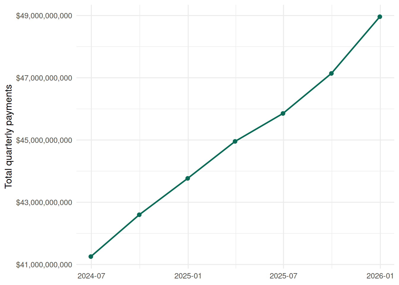
Across the visible payments extracts, observed NDIS payments increased by `r percent(overall_payment_growth, accuracy = 0.1)`, equivalent to about `r percent(overall_payment_quarterly_growth, accuracy = 0.1)` per quarter. This is a short window, so I treat it as the recent pace in the public files rather than a long-run trend.
```{r}
#| label: overall-payment-trend
#| fig-cap: "Total NDIS payments in the visible quarterly extracts."
if (nrow(overall_payment_trend) > 1) {
  ggplot(overall_payment_trend, aes(quarter_date, total_payments)) +
    geom_line(linewidth = 0.9, colour = "#0b6b57") +
    geom_point(size = 2, colour = "#0b6b57") +
    scale_y_continuous(labels = dollar) +
    labs(x = NULL, y = "Total quarterly payments")
} else {
  tibble(note = "Not enough payment quarters to draw the total spend chart.") |> kable()
}
```
## How Fast Is Participation Growing?
Before modelling budgets or utilisation, the first question is scale: is NDIS participation growing faster than the Australian population? The table below compares national NDIS participant counts from the public participant budget extract with ABS estimated resident population. The ABS quarterly population release currently overlaps the NDIS analysis window through September 2025, so the December 2025 NDIS quarter is not used in this comparison.
```{r}
#| label: population-participation-data
abs_population <- tibble::tribble(
  ~quarter_label, ~quarter_date, ~australian_population,
  "March 2024", "2024-03-31", 27113517,
  "June 2024", "2024-06-30", 27194286,
  "September 2024", "2024-09-30", 27301149,
  "December 2024", "2024-12-31", 27388133,
  "March 2025", "2025-03-31", 27531443,
  "June 2025", "2025-06-30", 27613654,
  "September 2025", "2025-09-30", 27724744
) |>
  mutate(
    quarter_date = as.Date(quarter_date),
    population_source = "ABS National, state and territory population, September 2025 release"
  )

population_participation <- national_participants |>
  inner_join(abs_population, by = c("quarter_label", "quarter_date")) |>
  arrange(quarter_date) |>
  mutate(
    ndis_share_population = ndis_participants / australian_population,
    ndis_participant_growth = ndis_participants / first(ndis_participants) - 1,
    population_growth = australian_population / first(australian_population) - 1,
    share_change_percentage_points = (ndis_share_population - first(ndis_share_population)) * 100
  )

participation_summary <- if (nrow(population_participation) > 0) {
  population_participation |>
    summarise(
      start_quarter = first(quarter_label),
      end_quarter = last(quarter_label),
      population_growth = last(population_growth),
      ndis_participant_growth = last(ndis_participant_growth),
      start_share = first(ndis_share_population),
      end_share = last(ndis_share_population)
    )
} else {
  tibble(
    start_quarter = NA_character_,
    end_quarter = NA_character_,
    population_growth = NA_real_,
    ndis_participant_growth = NA_real_,
    start_share = NA_real_,
    end_share = NA_real_
  )
}

if (nrow(population_participation) > 0) {
  population_participation |>
    transmute(
      quarter = quarter_label,
      australian_population = comma(australian_population),
      ndis_participants = comma(ndis_participants),
      population_growth = percent(population_growth, accuracy = 0.1),
      ndis_participant_growth = percent(ndis_participant_growth, accuracy = 0.1),
      ndis_share_population = percent(ndis_share_population, accuracy = 0.01),
      share_change_percentage_points = number(share_change_percentage_points, accuracy = 0.01)
    ) |>
    kable()
} else {
  tibble(note = "National NDIS participant counts could not be aligned to the ABS population denominator in this render.") |>
    kable()
}
```
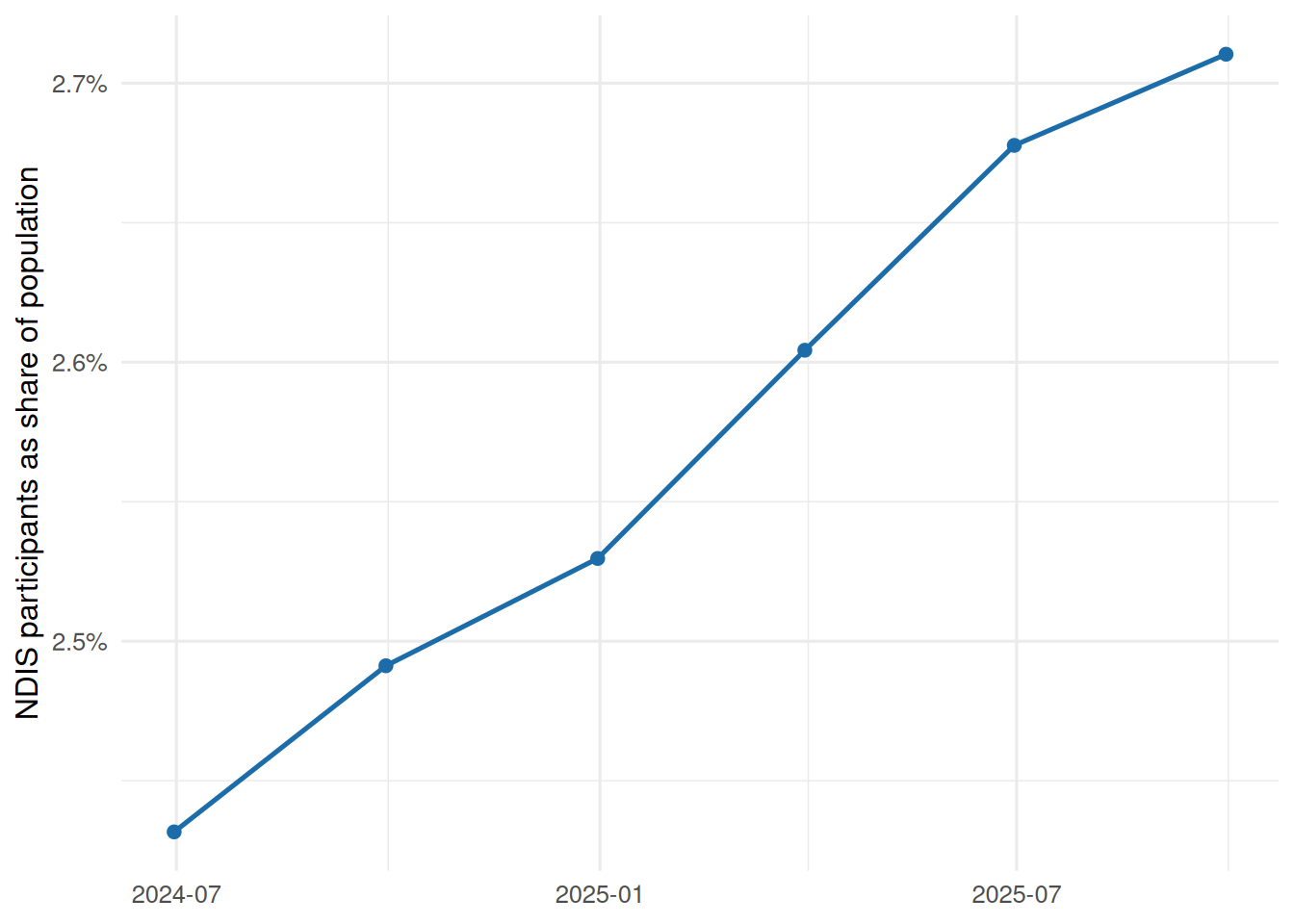
Over the overlapping ABS and NDIS window, the Australian population grew `r percent(participation_summary$population_growth, accuracy = 0.1)` while NDIS participant counts grew `r percent(participation_summary$ndis_participant_growth, accuracy = 0.1)`. That lifted observed NDIS participation from `r percent(participation_summary$start_share, accuracy = 0.01)` of the population in `r participation_summary$start_quarter` to `r percent(participation_summary$end_share, accuracy = 0.01)` by `r participation_summary$end_quarter`.
```{r}
#| label: population-participation-trend
#| fig-cap: "NDIS participant growth compared with Australian population growth, indexed to March 2024."
if (nrow(population_participation) > 1) {
  population_participation |>
    select(quarter_date, population_growth, ndis_participant_growth) |>
    pivot_longer(
      c(population_growth, ndis_participant_growth),
      names_to = "series",
      values_to = "growth"
    ) |>
    mutate(
      series = recode(
        series,
        population_growth = "Australian population",
        ndis_participant_growth = "NDIS participants"
      )
    ) |>
    ggplot(aes(quarter_date, growth, colour = series)) +
    geom_hline(yintercept = 0, colour = "grey80") +
    geom_line(linewidth = 0.9) +
    geom_point(size = 2) +
    scale_y_continuous(labels = percent) +
    labs(x = NULL, y = "Growth since March 2024", colour = NULL)
} else {
  tibble(note = "Not enough overlapping population and NDIS quarters to draw the indexed growth chart.") |>
    kable()
}
```
```{r}
#| label: ndis-share-population-trend
#| fig-cap: "Share of the Australian population participating in the NDIS."
if (nrow(population_participation) > 1) {
  population_participation |>
    ggplot(aes(quarter_date, ndis_share_population)) +
    geom_line(linewidth = 0.9, colour = "#1b6ca8") +
    geom_point(size = 2, colour = "#1b6ca8") +
    scale_y_continuous(labels = percent) +
    labs(x = NULL, y = "NDIS participants as share of population")
} else {
  tibble(note = "Not enough overlapping population and NDIS quarters to draw the participation-share chart.") |>
    kable()
}
```
```{r}
#| label: budget-trend
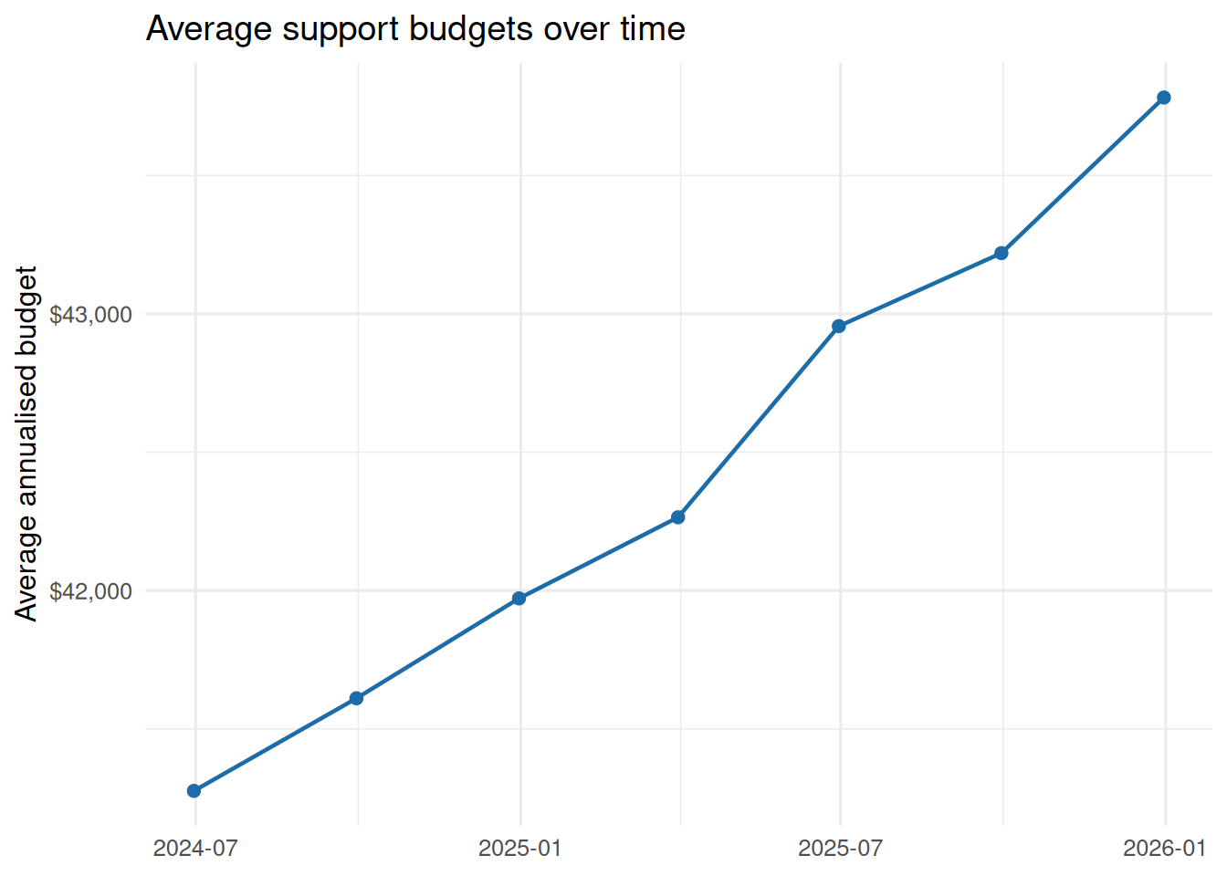
#| fig-cap: "Average support budget and participant counts across the visible quarterly extracts."
budget_trend_data <- budget |>
  group_by(quarter_date) |>
  summarise(
    participants = sum(participant_count, na.rm = TRUE),
    avg_budget = safe_weighted_mean(avg_support_budget, participant_count),
    .groups = "drop"
  ) |>
  filter(!is.na(avg_budget))

if (has_enough_data(budget_trend_data, c("avg_budget"))) {
  ggplot(budget_trend_data, aes(quarter_date, avg_budget)) +
    geom_line(linewidth = 0.8, colour = "#1b6ca8") +
    geom_point(size = 2, colour = "#1b6ca8") +
    scale_y_continuous(labels = dollar) +
    labs(x = NULL, y = "Average annualised budget", title = "Average support budgets over time")
} else {
  tibble(note = "Not enough non-missing average budget data to draw the trend chart.") |> kable()
}
```
```{r}
#| label: utilisation-trend
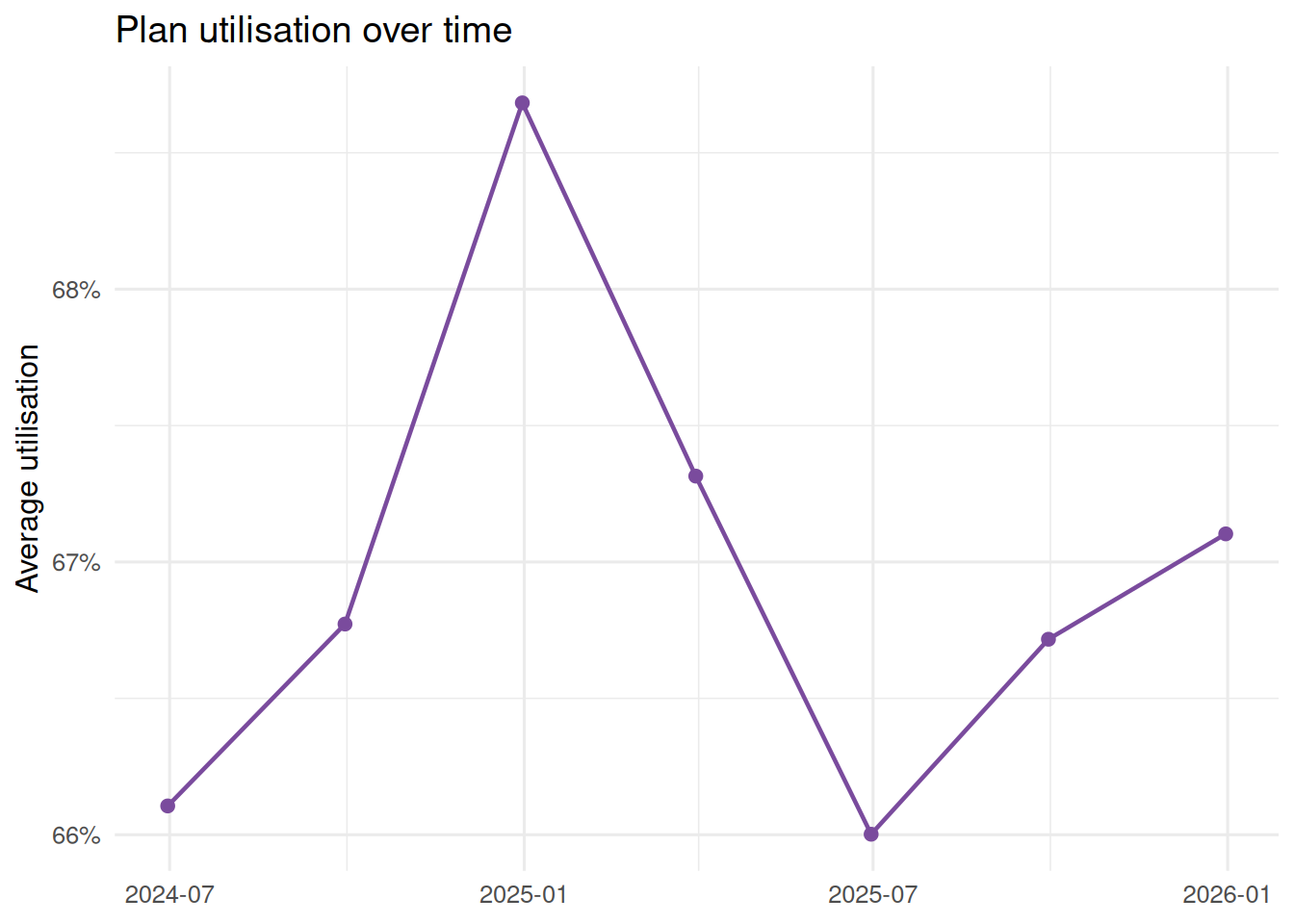
#| fig-cap: "Plan utilisation across the visible quarterly extracts."
utilisation_trend_data <- utilisation |>
  group_by(quarter_date) |>
  summarise(avg_utilisation = safe_mean(utilisation_rate), .groups = "drop") |>
  arrange(quarter_date)

utilisation_summary <- utilisation_trend_data |>
  summarise(
    start_utilisation = first(avg_utilisation),
    end_utilisation = last(avg_utilisation),
    min_utilisation = min(avg_utilisation, na.rm = TRUE),
    max_utilisation = max(avg_utilisation, na.rm = TRUE)
  )

utilisation_trend_data |>
  ggplot(aes(quarter_date, avg_utilisation)) +
  geom_line(linewidth = 0.8, colour = "#7a4b9d") +
  geom_point(size = 2, colour = "#7a4b9d") +
  scale_y_continuous(labels = percent) +
  labs(x = NULL, y = "Average utilisation", title = "Plan utilisation over time")
```
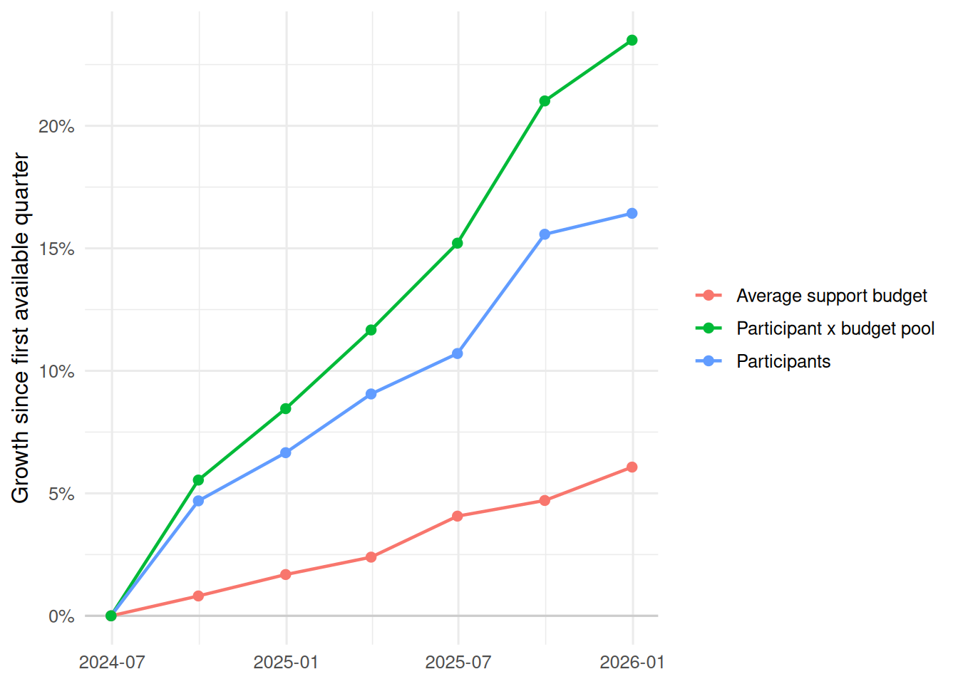
Payments are approximately participants multiplied by approved budgets multiplied by utilisation. In this short series, utilisation moves from `r percent(utilisation_summary$start_utilisation, accuracy = 0.1)` to `r percent(utilisation_summary$end_utilisation, accuracy = 0.1)`, with a range of `r percent(utilisation_summary$min_utilisation, accuracy = 0.1)` to `r percent(utilisation_summary$max_utilisation, accuracy = 0.1)`. That points the descriptive story toward participant growth and average budget growth rather than a large utilisation-rate shift.
```{r}
#| label: participant-budget-growth
#| fig-cap: "Participant count and average support budget growth, indexed to the first available quarter."
budget_pressure <- budget |>
  group_by(quarter_date) |>
  summarise(
    participants = sum(participant_count, na.rm = TRUE),
    avg_budget = safe_weighted_mean(avg_support_budget, participant_count),
    implied_budget_pool = sum(participant_count * avg_support_budget, na.rm = TRUE),
    .groups = "drop"
  ) |>
  arrange(quarter_date) |>
  mutate(
    participant_growth = participants / first(participants) - 1,
    avg_budget_growth = avg_budget / first(avg_budget) - 1,
    implied_pool_growth = implied_budget_pool / first(implied_budget_pool) - 1
  )

budget_pressure |>
  select(quarter_date, participant_growth, avg_budget_growth, implied_pool_growth) |>
  pivot_longer(-quarter_date, names_to = "measure", values_to = "growth") |>
  mutate(
    measure = recode(
      measure,
      participant_growth = "Participants",
      avg_budget_growth = "Average support budget",
      implied_pool_growth = "Participant x budget pool"
    )
  ) |>
  ggplot(aes(quarter_date, growth, colour = measure)) +
  geom_hline(yintercept = 0, colour = "grey80") +
  geom_line(linewidth = 0.8) +
  geom_point(size = 2) +
  scale_y_continuous(labels = percent) +
  labs(x = NULL, y = "Growth since first available quarter", colour = NULL)
```
::: {.callout-note collapse="true" title="Appendix: support-class budget snapshot"}
```{r}
#| label: support-class-summary
budget |>
  filter(quarter_date == max(quarter_date, na.rm = TRUE)) |>
  group_by(support_class) |>
  summarise(
    rows = n(),
    usable_participants = sum(participant_count, na.rm = TRUE),
    median_avg_budget = safe_median(avg_support_budget),
    mean_avg_budget = safe_mean(avg_support_budget),
    .groups = "drop"
  ) |>
  left_join(
    payments_support_class |>
      filter(quarter_date == max(quarter_date, na.rm = TRUE)) |>
      group_by(support_class) |>
      summarise(total_payments = sum(payment_amount, na.rm = TRUE), .groups = "drop"),
    by = "support_class"
  ) |>
  arrange(desc(total_payments)) |>
  mutate(
    usable_participants = comma(usable_participants),
    median_avg_budget = dollar(median_avg_budget, accuracy = 1),
    mean_avg_budget = dollar(mean_avg_budget, accuracy = 1),
    total_payments = dollar(total_payments, accuracy = 1)
  ) |>
  kable()
```
Suppressed participant counts such as `<11` are treated as missing. Weighted summaries use non-suppressed participant counts where they are available and otherwise fall back to unweighted summaries.
:::
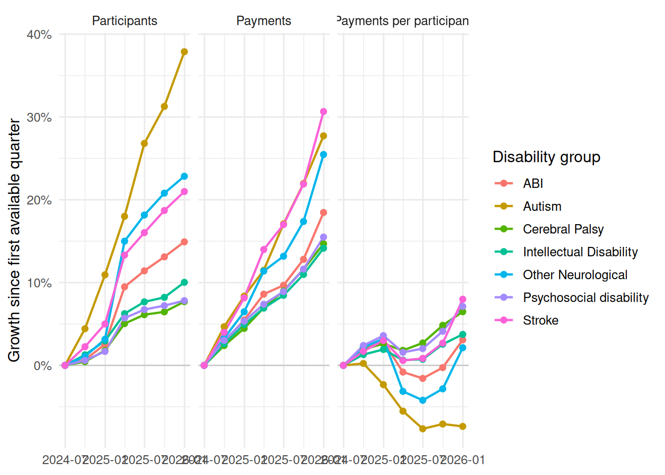
## Disability Mix and Payment Growth
The payments files are the most useful addition for spend analysis because they contain actual payment amounts by disability group as well as support class, support category, item, region and age band. The disability-group rows below use national aggregate rows where available, so nested `ALL` rows are not double-counted.
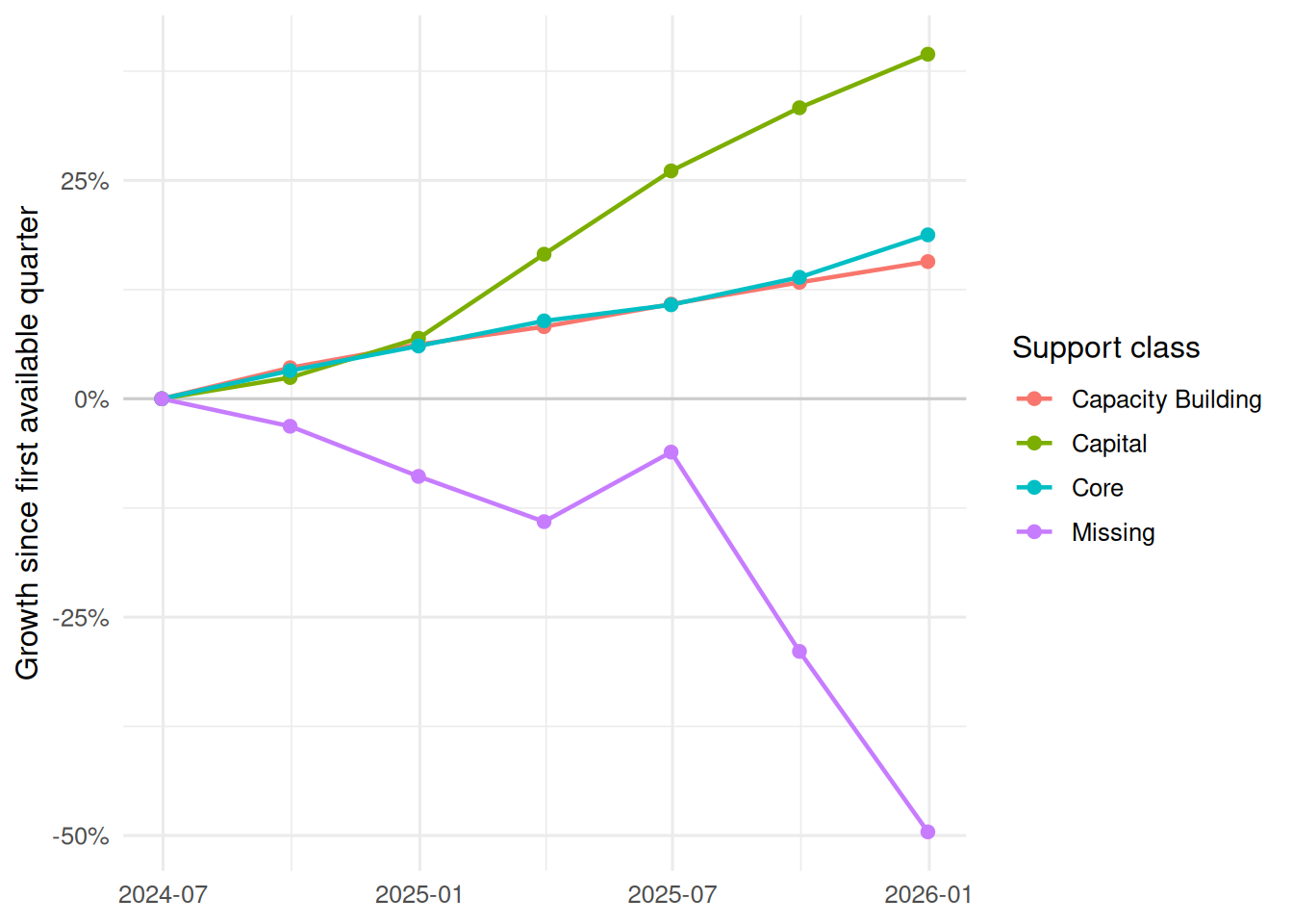
::: {.callout-note collapse="true" title="Appendix: support class, category and item payment growth"}
The support-level tables are still useful audit checks, but the main story below focuses on disability groups.
```{r}
#| label: payment-growth-overall
#| fig-cap: "Payment growth by support class, indexed to the first available quarter."
payments_support_class |>
  group_by(quarter_date, support_class) |>
  summarise(payment_amount = sum(payment_amount, na.rm = TRUE), .groups = "drop") |>
  group_by(support_class) |>
  arrange(quarter_date, .by_group = TRUE) |>
  mutate(index = payment_amount / first(payment_amount) - 1) |>
  ungroup() |>
  ggplot(aes(quarter_date, index, colour = support_class)) +
  geom_hline(yintercept = 0, colour = "grey80") +
  geom_line(linewidth = 0.8) +
  geom_point(size = 2) +
  scale_y_continuous(labels = percent) +
  labs(x = NULL, y = "Growth since first available quarter", colour = "Support class")
```
```{r}
#| label: support-class-growth-contribution
first_payment_qtr <- min(payments_support_class$quarter_date, na.rm = TRUE)
last_payment_qtr <- max(payments_support_class$quarter_date, na.rm = TRUE)

payment_change <- function(data, group_vars) {
  if (nrow(data) == 0) {
    return(tibble(
      !!!set_names(rep(list(character()), length(group_vars)), group_vars),
      payment_amount_first = numeric(),
      payment_amount_last = numeric(),
      participants_first = numeric(),
      participants_last = numeric(),
      payment_change = numeric(),
      participant_change = numeric(),
      payment_per_participant_first = numeric(),
      payment_per_participant_last = numeric(),
      payment_per_participant_change = numeric()
    ))
  }

  wide <- data |>
    filter(quarter_date %in% c(first_payment_qtr, last_payment_qtr)) |>
    group_by(across(all_of(group_vars)), quarter_date) |>
    summarise(
      payment_amount = sum(payment_amount, na.rm = TRUE),
      participants = sum(payment_participants, na.rm = TRUE),
      .groups = "drop"
    ) |>
    mutate(period = if_else(quarter_date == first_payment_qtr, "first", "last")) |>
    select(-quarter_date) |>
    pivot_wider(
      names_from = period,
      values_from = c(payment_amount, participants),
      values_fill = 0
    )

  needed_cols <- c("payment_amount_first", "payment_amount_last", "participants_first", "participants_last")
  for (col in needed_cols) {
    if (!col %in% names(wide)) wide[[col]] <- 0
  }

  wide |>
    mutate(
      payment_amount_first = coalesce(payment_amount_first, 0),
      payment_amount_last = coalesce(payment_amount_last, 0),
      participants_first = coalesce(participants_first, 0),
      participants_last = coalesce(participants_last, 0),
      payment_change = payment_amount_last - payment_amount_first,
      participant_change = participants_last - participants_first,
      payment_per_participant_first = payment_amount_first / participants_first,
      payment_per_participant_last = payment_amount_last / participants_last,
      payment_per_participant_change = payment_per_participant_last - payment_per_participant_first
    ) |>
    arrange(desc(abs(payment_change)))
}

support_class_change <- payment_change(payments_support_class, "support_class")

support_class_change |>
  mutate(
    across(c(payment_amount_first, payment_amount_last, payment_change), \(x) dollar(x, accuracy = 1)),
    across(c(participants_first, participants_last, participant_change), comma),
    across(c(payment_per_participant_first, payment_per_participant_last, payment_per_participant_change), \(x) dollar(x, accuracy = 1))
  ) |>
  kable()
```
```{r}
#| label: category-growth-contribution
category_change <- payment_change(payments_category, c("support_class", "support_category"))

category_change |>
  slice_max(abs(payment_change), n = 15) |>
  mutate(
    payment_change = dollar(payment_change, accuracy = 1),
    payment_amount_last = dollar(payment_amount_last, accuracy = 1),
    participant_change = comma(participant_change),
    payment_per_participant_change = dollar(payment_per_participant_change, accuracy = 1)
  ) |>
  select(support_class, support_category, payment_amount_last, payment_change, participant_change, payment_per_participant_change) |>
  kable()
```
```{r}
#| label: item-growth-contribution
item_change <- payment_change(payments_item, c("support_class", "support_category", "support_item_number", "support_item_desc"))

if (nrow(item_change) > 0) {
  item_change |>
    slice_max(abs(payment_change), n = 15) |>
    mutate(
      support_item_desc = str_trunc(support_item_desc, 70),
      payment_amount_last = dollar(payment_amount_last, accuracy = 1),
      payment_change = dollar(payment_change, accuracy = 1),
      participant_change = comma(participant_change),
      payment_per_participant_change = dollar(payment_per_participant_change, accuracy = 1)
    ) |>
    select(support_class, support_category, support_item_number, support_item_desc, payment_amount_last, payment_change, participant_change, payment_per_participant_change) |>
    kable()
} else {
  tibble(note = "The current public payments extract did not expose national item-level rows under the no-double-counting filters used here.") |>
    kable()
}
```
:::
```{r}
#| label: disability-payment-driver-data
payments_disability_candidates <- payments |>
  filter(
    state == "ALL", service_district == "ALL", disability_group != "ALL", age_group == "ALL",
    support_category == "ALL", support_item_number == "ALL"
  )

if (any(payments_disability_candidates$support_class == "ALL", na.rm = TRUE)) {
  payments_disability <- payments_disability_candidates |>
    filter(support_class == "ALL") |>
    group_by(quarter_label, quarter_date, quarter_index, disability_group) |>
    summarise(
      payment_amount = sum(payment_amount, na.rm = TRUE),
      payment_participants = max(payment_participants, na.rm = TRUE),
      .groups = "drop"
    )
  disability_payment_basis <- "National disability-group aggregate rows"
} else {
  payments_disability <- payments_disability_candidates |>
    filter(support_class != "ALL") |>
    group_by(quarter_label, quarter_date, quarter_index, disability_group) |>
    summarise(
      payment_amount = sum(payment_amount, na.rm = TRUE),
      payment_participants = sum(payment_participants, na.rm = TRUE),
      .groups = "drop"
    )
  disability_payment_basis <- "Support-class rows summed within disability group"
}

payments_disability <- payments_disability |>
  mutate(
    payment_participants = if_else(is.infinite(payment_participants), NA_real_, payment_participants),
    payment_per_participant = payment_amount / payment_participants
  )

tibble(
  basis = disability_payment_basis,
  disability_groups = n_distinct(payments_disability$disability_group),
  quarters = paste(sort(unique(payments_disability$quarter_label)), collapse = ", ")
) |>
  kable()
```
```{r}
#| label: disability-group-snapshot
#| include: false
latest_disability_snapshot <- payments_disability |>
filter(quarter_date == max(quarter_date, na.rm = TRUE)) |>
mutate(payment_per_participant = payment_amount / payment_participants)
largest_by_count <- latest_disability_snapshot |>
slice_max(payment_participants, n = 10, with_ties = FALSE)
largest_by_spend <- latest_disability_snapshot |>
slice_max(payment_amount, n = 10, with_ties = FALSE)
largest_by_average_spend <- latest_disability_snapshot |>
filter(payment_participants >= quantile(payment_participants, 0.25, na.rm = TRUE)) |>
slice_max(payment_per_participant, n = 10, with_ties = FALSE)
```
The participant-count view shows scale: groups that are large enough to move total spend even if average payments are moderate.
```{r}
#| label: disability-largest-by-count
largest_by_count |>
  transmute(
    disability_group,
    payment_participants = comma(payment_participants),
    total_payments = dollar(payment_amount, accuracy = 1),
    payment_per_participant = dollar(payment_per_participant, accuracy = 1)
  ) |>
  kable()
```
The total-payments view combines scale and intensity: these are the groups contributing the largest payment dollars in the latest quarter.
```{r}
#| label: disability-largest-by-total-payments
largest_by_spend |>
  transmute(
    disability_group,
    total_payments = dollar(payment_amount, accuracy = 1),
    payment_participants = comma(payment_participants),
    payment_per_participant = dollar(payment_per_participant, accuracy = 1)
  ) |>
  kable()
```
The average-payment view is filtered to groups above the first quartile of participant counts, so it does not get dominated by very small groups with noisy averages.
```{r}
#| label: disability-highest-average-payment
largest_by_average_spend |>
  transmute(
    disability_group,
    payment_per_participant = dollar(payment_per_participant, accuracy = 1),
    payment_participants = comma(payment_participants),
    total_payments = dollar(payment_amount, accuracy = 1)
  ) |>
  kable()
```
```{r}
#| label: disability-driver-decomposition
disability_change <- payment_change(payments_disability, "disability_group")

total_disability_payment_change <- sum(disability_change$payment_change, na.rm = TRUE)

disability_driver <- disability_change |>
  mutate(
    participant_contribution = (participants_last - participants_first) *
      ((payment_per_participant_first + payment_per_participant_last) / 2),
    intensity_contribution = (payment_per_participant_last - payment_per_participant_first) *
      ((participants_first + participants_last) / 2),
    change_share = payment_change / total_disability_payment_change,
    stroke_flag = str_detect(str_to_lower(disability_group), "\\bstroke\\b")
  ) |>
  arrange(desc(abs(payment_change)))

if (nrow(disability_driver) > 0) {
  disability_driver |>
    slice_max(abs(payment_change), n = 15) |>
    transmute(
      disability_group,
      payment_amount_last = dollar(payment_amount_last, accuracy = 1),
      payment_change = dollar(payment_change, accuracy = 1),
      change_share = percent(change_share, accuracy = 0.1),
      participant_change = comma(participant_change),
      participant_contribution = dollar(participant_contribution, accuracy = 1),
      intensity_contribution = dollar(intensity_contribution, accuracy = 1),
      payment_per_participant_change = dollar(payment_per_participant_change, accuracy = 1)
    ) |>
    kable()
} else {
  tibble(note = "No disability-group payment rows were available under the no-double-counting filters used here.") |>
    kable()
}
```
```{r}
#| label: disability-driver-trends
#| fig-cap: "Payment, participant and payment-per-participant trends for stroke and the largest disability-group growth contributors."
top_driver_groups <- disability_driver |>
  filter(is.finite(payment_change)) |>
  slice_max(abs(payment_change), n = 7) |>
  pull(disability_group)

stroke_groups <- disability_driver |>
  filter(stroke_flag) |>
  pull(disability_group)

driver_groups <- unique(c(stroke_groups, top_driver_groups)) |>
  head(8)

disability_trend <- payments_disability |>
  filter(disability_group %in% driver_groups) |>
  arrange(disability_group, quarter_date) |>
  group_by(disability_group) |>
  mutate(
    payment_growth = index_to_first(payment_amount),
    participant_growth = index_to_first(payment_participants),
    payment_per_participant_growth = index_to_first(payment_per_participant)
  ) |>
  ungroup()

if (nrow(disability_trend) > 0) {
  disability_trend |>
    select(quarter_date, disability_group, payment_growth, participant_growth, payment_per_participant_growth) |>
    pivot_longer(
      ends_with("_growth"),
      names_to = "measure",
      values_to = "growth"
    ) |>
    mutate(
      measure = recode(
        measure,
        payment_growth = "Payments",
        participant_growth = "Participants",
        payment_per_participant_growth = "Payments per participant"
      )
    ) |>
    filter(is.finite(growth)) |>
    ggplot(aes(quarter_date, growth, colour = disability_group)) +
    geom_hline(yintercept = 0, colour = "grey80") +
    geom_line(linewidth = 0.8) +
    geom_point(size = 1.8) +
    facet_wrap(~ measure) +
    scale_y_continuous(labels = percent) +
    labs(x = NULL, y = "Growth since first available quarter", colour = "Disability group")
} else {
  tibble(note = "No stroke or top-driver disability-group trend rows were available to plot.") |>
    kable()
}
```
```{r}
#| label: stroke-driver-summary
if (any(disability_driver$stroke_flag, na.rm = TRUE)) {
  disability_driver |>
    filter(stroke_flag) |>
    transmute(
      disability_group,
      payment_amount_first = dollar(payment_amount_first, accuracy = 1),
      payment_amount_last = dollar(payment_amount_last, accuracy = 1),
      payment_change = dollar(payment_change, accuracy = 1),
      change_share = percent(change_share, accuracy = 0.1),
      participants_first = comma(participants_first),
      participants_last = comma(participants_last),
      participant_change = comma(participant_change),
      payment_per_participant_change = dollar(payment_per_participant_change, accuracy = 1)
    ) |>
    kable()
} else {
  tibble(note = "Stroke was not exposed as a separate disability group in the current public payment extract.") |>
    kable()
}
```
The payment tables are useful, but the time window is short. These are growth-contribution signals, not stable long-run trends. The disability-group decomposition separates participant growth from payment intensity, but it still reflects aggregate public payment rows rather than participant-level need or plan history.
::: {.callout-note collapse="true" title="Appendix: budgets, payments and utilisation detail"}
## Budgets, Payments and Utilisation
Budget, utilisation and payments answer related but different questions. A high annualised support budget does not necessarily mean a high payment amount in the observed quarter, and low utilisation can reflect need, timing, provider availability or administrative barriers.
```{r}
#| label: budget-payment-utilisation-data
latest_model_data <- model_data |>
  filter(quarter_date == max(quarter_date, na.rm = TRUE)) |>
  filter(!is.na(avg_support_budget), !is.na(utilisation_rate), !is.na(payment_amount), !is.na(payment_per_participant)) |>
  mutate(
    utilisation_rate = pmin(utilisation_rate, 1),
    high_budget_cut = quantile(avg_support_budget, 0.75, na.rm = TRUE),
    low_utilisation_cut = quantile(utilisation_rate, 0.25, na.rm = TRUE),
    high_utilisation_cut = quantile(utilisation_rate, 0.75, na.rm = TRUE),
    high_payment_cut = quantile(payment_per_participant, 0.75, na.rm = TRUE),
    signal = case_when(
      avg_support_budget >= high_budget_cut & utilisation_rate <= low_utilisation_cut ~ "High budget, low utilisation",
      utilisation_rate >= high_utilisation_cut & payment_per_participant >= high_payment_cut ~ "High utilisation, high payment",
      payment_per_participant >= high_payment_cut & avg_support_budget < high_budget_cut ~ "High payment, moderate budget",
      TRUE ~ NA_character_
    )
  )
```
```{r}
#| label: budget-payment-utilisation-definitions
tibble(
  signal = c("High budget, low utilisation", "High utilisation, high payment", "High payment, moderate budget"),
  definition = c(
    "Average support budget is in the top quartile while utilisation is in the bottom quartile.",
    "Utilisation and payments per participant are both in the top quartile.",
    "Payments per participant are in the top quartile while average support budget is below the top quartile."
  )
) |>
  kable()
```
```{r}
#| label: budget-payment-utilisation-signal-summary
signal_data <- latest_model_data |>
  filter(!is.na(signal))

signal_data |>
  group_by(signal) |>
  summarise(
    service_districts = n_distinct(service_district),
    grouped_cells = n(),
    participants = sum(participant_count, na.rm = TRUE),
    total_payments = sum(payment_amount, na.rm = TRUE),
    median_payment_per_participant = safe_median(payment_per_participant),
    median_utilisation = safe_median(utilisation_rate),
    median_avg_budget = safe_median(avg_support_budget),
    .groups = "drop"
  ) |>
  mutate(
    participants = comma(participants),
    total_payments = dollar(total_payments, accuracy = 1),
    median_payment_per_participant = dollar(median_payment_per_participant, accuracy = 1),
    median_utilisation = percent(median_utilisation, accuracy = 0.1),
    median_avg_budget = dollar(median_avg_budget, accuracy = 1)
  ) |>
  kable()
```
```{r}
#| label: budget-payment-utilisation-top-signals
signal_data |>
  group_by(signal, state, service_district, support_class) |>
  summarise(
    grouped_cells = n(),
    participants = sum(participant_count, na.rm = TRUE),
    total_payments = sum(payment_amount, na.rm = TRUE),
    median_utilisation = safe_median(utilisation_rate),
    median_payment_per_participant = safe_median(payment_per_participant),
    .groups = "drop"
  ) |>
  arrange(signal, desc(participants)) |>
  group_by(signal) |>
  slice_head(n = 5) |>
  ungroup() |>
  mutate(
    participants = comma(participants),
    total_payments = dollar(total_payments, accuracy = 1),
    median_utilisation = percent(median_utilisation, accuracy = 0.1),
    median_payment_per_participant = dollar(median_payment_per_participant, accuracy = 1)
  ) |>
  kable()
```
:::
::: {.callout-note collapse="true" title="Appendix: provider market context"}
## Provider Market Context
Provider-market context is one of the few public levers that can plausibly help explain utilisation. The measures below are deliberately rough. `participants_per_provider` is a demand-pressure proxy, while `payment_share_top10` is a concentration proxy. Neither measures provider quality, available hours, wait time, travel burden or workforce depth.
```{r}
#| label: provider-context-table
latest_model_data |>
  group_by(support_class) |>
  summarise(
    grouped_cells = n(),
    participants = sum(participant_count, na.rm = TRUE),
    median_utilisation = safe_median(utilisation_rate),
    median_participants_per_provider = safe_median(participants_per_provider),
    median_payment_share_top10 = safe_median(payment_share_top10),
    median_payment_per_participant = safe_median(payment_per_participant),
    .groups = "drop"
  ) |>
  mutate(
    participants = comma(participants),
    median_utilisation = percent(median_utilisation, accuracy = 0.1),
    median_participants_per_provider = number(median_participants_per_provider, accuracy = 0.1),
    median_payment_share_top10 = percent(median_payment_share_top10, accuracy = 0.1),
    median_payment_per_participant = dollar(median_payment_per_participant, accuracy = 1)
  ) |>
  kable()
```
```{r}
#| label: provider-context-quadrants
provider_quadrant_data <- latest_model_data |>
  filter(is.finite(participants_per_provider), is.finite(payment_share_top10)) |>
  mutate(
    provider_pressure = if_else(participants_per_provider >= safe_median(participants_per_provider), "High provider pressure", "Low provider pressure"),
    concentration = if_else(payment_share_top10 >= safe_median(payment_share_top10), "High concentration", "Low concentration"),
    quadrant = paste(provider_pressure, concentration, sep = " / ")
  )

provider_quadrant_data |>
  group_by(quadrant) |>
  summarise(
    service_districts = n_distinct(service_district),
    grouped_cells = n(),
    participants = sum(participant_count, na.rm = TRUE),
    median_utilisation = safe_median(utilisation_rate),
    median_payment_per_participant = safe_median(payment_per_participant),
    median_payment_share_top10 = safe_median(payment_share_top10),
    .groups = "drop"
  ) |>
  mutate(
    participants = comma(participants),
    median_utilisation = percent(median_utilisation, accuracy = 0.1),
    median_payment_per_participant = dollar(median_payment_per_participant, accuracy = 1),
    median_payment_share_top10 = percent(median_payment_share_top10, accuracy = 0.1)
  ) |>
  kable()
```
:::
## SIL and SDA Baseline
The utilisation extract includes a `SILorSDA` field. That makes it possible to set a pre-reform descriptive baseline before mandatory registration for supported independent living and platform providers begins on [1 July 2026](https://www.ndiscommission.gov.au/about-us/ndis-commission-reform-hub/mandatory-registration). This is not an evaluation of that change; it is a baseline view of utilisation patterns before the reform takes effect.
```{r}
#| label: sil-sda-utilisation
sil_sda_utilisation <- utilisation |>
  filter(!is.na(sil_or_sda), sil_or_sda != "ALL", support_class != "ALL") |>
  group_by(quarter_date, sil_or_sda, support_class) |>
  summarise(utilisation = safe_mean(utilisation_rate), rows = n(), .groups = "drop")

sil_sda_utilisation |>
  ggplot(aes(quarter_date, utilisation, colour = sil_or_sda)) +
  geom_line(linewidth = 0.8) +
  geom_point(size = 2) +
  facet_wrap(~ support_class) +
  scale_y_continuous(labels = percent) +
  labs(x = NULL, y = "Average utilisation", colour = "SIL/SDA flag")
```
```{r}
#| label: sil-sda-payments
sil_sda_payment_items <- payments_item |>
  filter(str_detect(str_to_lower(paste(support_category, support_item_desc)), "supported independent living|\\bsil\\b|specialist disability accommodation|\\bsda\\b"))

if (nrow(sil_sda_payment_items) > 0) {
  sil_sda_payment_items |>
    group_by(quarter_date, support_class, support_category) |>
    summarise(payment_amount = sum(payment_amount, na.rm = TRUE), participants = sum(payment_participants, na.rm = TRUE), .groups = "drop") |>
    arrange(desc(payment_amount)) |>
    mutate(
      payment_amount = dollar(payment_amount, accuracy = 1),
      participants = comma(participants)
    ) |>
    slice_head(n = 15) |>
    kable()
} else {
  tibble(note = "No payment item descriptions matched SIL/SDA keywords in the national item-level extract.") |>
    kable()
}
```
::: {.callout-note collapse="true" title="Appendix: regional context and join quality"}
## Regional Context and Join Quality
The regional layer is deliberately conservative. It uses the NDIS service-district-to-LGA mapping, then joins ABS LGA SEIFA, age-structure, population, and remoteness allocation files where the source workbooks resolve cleanly. Remoteness is allocated from ABS mesh-block and SA1 correspondence files up to LGA, then aggregated to service districts with population weights. The table below keeps the join quality visible so the model does not quietly imply more geographic precision than the data supports.
```{r}
#| label: regional-join-quality
join_diagnostics |>
  mutate(coverage = percent(coverage, accuracy = 0.1)) |>
  kable()
```
```{r}
#| label: regional-context-table
model_data |>
  filter(quarter_date == max(quarter_date, na.rm = TRUE)) |>
  group_by(state, service_district) |>
  summarise(
    participants = sum(participant_count, na.rm = TRUE),
    avg_budget = safe_weighted_mean(avg_support_budget, participant_count),
    utilisation = safe_weighted_mean(utilisation_rate, participant_count),
    payment_per_participant = safe_weighted_mean(payment_per_participant, participant_count),
    participants_per_provider = safe_weighted_mean(participants_per_provider, participant_count),
    payment_share_top10 = safe_mean(payment_share_top10),
    remoteness = safe_mode_character(remoteness),
    irsd_decile = safe_mean(irsd_decile),
    median_age = safe_mean(median_age),
    pct_65_plus = safe_mean(pct_65_plus),
    mapped_lgas = max(mapped_lgas, na.rm = TRUE),
    .groups = "drop"
  ) |>
  arrange(desc(participants)) |>
  slice_head(n = 20) |>
  mutate(
    participants = comma(participants),
    avg_budget = dollar(avg_budget, accuracy = 1),
    utilisation = percent(utilisation, accuracy = 0.1),
    payment_per_participant = dollar(payment_per_participant, accuracy = 1),
    participants_per_provider = number(participants_per_provider, accuracy = 0.1),
    payment_share_top10 = percent(payment_share_top10, accuracy = 0.1),
    irsd_decile = number(irsd_decile, accuracy = 0.1),
    median_age = number(median_age, accuracy = 0.1),
    pct_65_plus = number(pct_65_plus, accuracy = 0.1, suffix = "%"),
    mapped_lgas = comma(mapped_lgas)
  ) |>
  kable()
```
```{r}
#| label: service-district-geography-profile
latest_service_geo <- model_data |>
  filter(quarter_date == max(quarter_date, na.rm = TRUE)) |>
  group_by(state, service_district) |>
  summarise(
    participants = sum(participant_count, na.rm = TRUE),
    avg_budget = safe_weighted_mean(avg_support_budget, participant_count),
    utilisation = safe_weighted_mean(utilisation_rate, participant_count),
    payment_per_participant = safe_weighted_mean(payment_per_participant, participant_count),
    participants_per_provider = safe_weighted_mean(participants_per_provider, participant_count),
    payment_share_top10 = safe_mean(payment_share_top10),
    remoteness = safe_mode_character(remoteness),
    mapped_lgas = max(mapped_lgas, na.rm = TRUE),
    example_lgas = safe_mode_character(mapped_lga_names),
    irsd_decile = safe_mean(irsd_decile),
    median_age = safe_mean(median_age),
    pct_65_plus = safe_mean(pct_65_plus),
    .groups = "drop"
  ) |>
  mutate(
    mapped_lgas = if_else(is.infinite(mapped_lgas), NA_real_, as.numeric(mapped_lgas)),
    participant_rank = percent_rank(participants),
    budget_rank = percent_rank(avg_budget),
    payment_rank = percent_rank(payment_per_participant),
    utilisation_rank = percent_rank(utilisation),
    provider_pressure_rank = percent_rank(participants_per_provider),
    concentration_rank = percent_rank(payment_share_top10),
    geography_pressure_score = rowMeans(
      cbind(payment_rank, utilisation_rank, provider_pressure_rank, concentration_rank),
      na.rm = TRUE
    ),
    geography_pressure_score = if_else(is.nan(geography_pressure_score), NA_real_, geography_pressure_score)
  )

if (nrow(latest_service_geo) > 0) {
  latest_service_geo |>
    arrange(desc(geography_pressure_score), desc(participants)) |>
    slice_head(n = 15) |>
    transmute(
      state,
      service_district,
      remoteness,
      mapped_lgas = comma(mapped_lgas),
      participants = comma(participants),
      avg_budget = dollar(avg_budget, accuracy = 1),
      utilisation = percent(utilisation, accuracy = 0.1),
      payment_per_participant = dollar(payment_per_participant, accuracy = 1),
      participants_per_provider = number(participants_per_provider, accuracy = 0.1),
      payment_share_top10 = percent(payment_share_top10, accuracy = 0.1),
      irsd_decile = number(irsd_decile, accuracy = 0.1)
    ) |>
    kable()
} else {
  tibble(note = "No latest-quarter service-district geography profile could be built.") |>
    kable()
}
```
```{r}
#| label: remoteness-profile
remoteness_profile <- latest_service_geo |>
  filter(!is.na(remoteness))

if (nrow(remoteness_profile) > 0) {
  remoteness_profile |>
    group_by(remoteness) |>
    summarise(
      service_districts = n_distinct(service_district),
      participants = sum(participants, na.rm = TRUE),
      avg_budget = safe_weighted_mean(avg_budget, participants),
      utilisation = safe_weighted_mean(utilisation, participants),
      payment_per_participant = safe_weighted_mean(payment_per_participant, participants),
      participants_per_provider = safe_weighted_mean(participants_per_provider, participants),
      payment_share_top10 = safe_mean(payment_share_top10),
      median_irsd_decile = safe_median(irsd_decile),
      .groups = "drop"
    ) |>
    arrange(median_irsd_decile, desc(participants)) |>
    mutate(
      participants = comma(participants),
      avg_budget = dollar(avg_budget, accuracy = 1),
      utilisation = percent(utilisation, accuracy = 0.1),
      payment_per_participant = dollar(payment_per_participant, accuracy = 1),
      participants_per_provider = number(participants_per_provider, accuracy = 0.1),
      payment_share_top10 = percent(payment_share_top10, accuracy = 0.1),
      median_irsd_decile = number(median_irsd_decile, accuracy = 0.1)
    ) |>
    kable()
} else {
  tibble(note = "Remoteness was not available in the downloaded LGA mapping or participants-by-LGA file for this render.") |>
    kable()
}
```
:::
::: {.callout-note collapse="true" title="Appendix: richer geography context"}
## Richer Geography Context
The richer geography layer adds two lenses: socioeconomic decile where the ABS join works, and support-class market concentration. Equity-specific signals are left out of this version so the main post stays focused on spend growth mechanics.
```{r}
#| label: seifa-decile-summary
seifa_summary <- model_data |>
  filter(quarter_date == max(quarter_date, na.rm = TRUE), !is.na(irsd_decile))

if (nrow(seifa_summary) > 0) {
  seifa_summary |>
    mutate(irsd_decile = round(irsd_decile)) |>
    group_by(irsd_decile) |>
    summarise(
      participants = sum(participant_count, na.rm = TRUE),
      avg_budget = safe_weighted_mean(avg_support_budget, participant_count),
      utilisation = safe_weighted_mean(utilisation_rate, participant_count),
      payment_per_participant = safe_weighted_mean(payment_per_participant, participant_count),
      participants_per_provider = safe_weighted_mean(participants_per_provider, participant_count),
      payment_share_top10 = safe_mean(payment_share_top10),
      .groups = "drop"
    ) |>
    arrange(irsd_decile) |>
    mutate(
      participants = comma(participants),
      avg_budget = dollar(avg_budget, accuracy = 1),
      utilisation = percent(utilisation, accuracy = 0.1),
      payment_per_participant = dollar(payment_per_participant, accuracy = 1),
      participants_per_provider = number(participants_per_provider, accuracy = 0.1),
      payment_share_top10 = percent(payment_share_top10, accuracy = 0.1)
    ) |>
    kable()
} else {
  tibble(note = "SEIFA was not joined in this render, so the SEIFA decile summary is skipped rather than showing an NA-heavy table.") |>
    kable()
}
```
```{r}
#| label: market-concentration-by-support
market_concentration |>
  filter(market_quarter_date == max(market_quarter_date, na.rm = TRUE), support_class != "ALL") |>
  group_by(support_class) |>
  summarise(
    service_districts = n_distinct(service_district),
    median_top10_share = safe_median(payment_share_top10),
    high_concentration_share = safe_mean(as.numeric(payment_share_top10 >= 0.7)),
    .groups = "drop"
  ) |>
  arrange(desc(median_top10_share)) |>
  mutate(
    median_top10_share = percent(median_top10_share, accuracy = 0.1),
    high_concentration_share = percent(high_concentration_share, accuracy = 0.1)
  ) |>
  kable()
```
:::
## Outcomes, Spend and Service Access
The outcomes analysis has been moved into a separate companion post: [NDIS Outcomes, Spend and Service Access](../ndis-outcomes-spend-service-access/). That page inspects the regional dashboard workbook schema directly, chooses a small set of high-value outcome families, and treats outcomes as possible investment channels rather than only as cost offsets.
::: {.callout-note collapse="true" title="Appendix: average budget and utilisation model detail"}
## Model 1: Average Support Budget
The first model asks whether grouped participant characteristics, region, support class, provider supply, and ABS context explain differences in average support budgets. The expanded model now carries through service district plus joined LGA-level SEIFA, age-structure and population measures where the joins succeed. The test period is the latest available quarter in the study window, so the model is judged on a future quarter rather than a random split.
```{r}
#| label: budget-model
budget_model_data <- model_data |>
  filter(!is.na(avg_support_budget), !is.na(participant_count), participant_count > 0) |>
  mutate(
    across(c(state, service_district, age_group, disability_group, support_class, remoteness), \(x) fct_na_value_to_level(fct_lump_n(as.factor(x), n = 20), level = "Missing")),
    log_budget = log1p(avg_support_budget),
    log_participants = log1p(participant_count),
    log_providers = log1p(coalesce(active_providers, 0)),
    log_participants_per_provider = log1p(coalesce(participants_per_provider, 0)),
    log_lga_population = log1p(coalesce(lga_population, 0)),
    payment_share_top10 = coalesce(payment_share_top10, median(payment_share_top10, na.rm = TRUE)),
    payment_share_top10 = ifelse(is.na(payment_share_top10) | is.nan(payment_share_top10), 0, payment_share_top10),
    across(c(irsd_score, irsd_decile, ier_score, ier_decile, ieo_score, ieo_decile, median_age, pct_0_14, pct_15_64, pct_65_plus, remoteness_rank, remoteness_major_cities_share, remoteness_inner_regional_share, remoteness_outer_regional_share, remoteness_remote_share, remoteness_very_remote_share), \(x) replace_na(x, median(x, na.rm = TRUE))),
    across(c(irsd_score, irsd_decile, ier_score, ier_decile, ieo_score, ieo_decile, median_age, pct_0_14, pct_15_64, pct_65_plus, remoteness_rank, remoteness_major_cities_share, remoteness_inner_regional_share, remoteness_outer_regional_share, remoteness_remote_share, remoteness_very_remote_share), \(x) ifelse(is.na(x) | is.nan(x), 0, x))
  )

test_quarter <- max(budget_model_data$quarter_date, na.rm = TRUE)
budget_train <- filter(budget_model_data, quarter_date < test_quarter)
budget_test <- filter(budget_model_data, quarter_date == test_quarter)

budget_baseline <- lm(log_budget ~ quarter_index + log_participants, data = budget_train)

factor_terms <- c("state", "service_district", "age_group", "disability_group", "support_class", "remoteness")
factor_terms <- factor_terms[map_int(budget_train[factor_terms], \(x) n_distinct(x, na.rm = TRUE)) > 1]
numeric_terms <- c("quarter_index", "log_participants", "log_providers", "log_participants_per_provider", "payment_share_top10", "irsd_score", "irsd_decile", "ier_score", "ier_decile", "ieo_score", "ieo_decile", "median_age", "pct_0_14", "pct_15_64", "pct_65_plus", "log_lga_population", "remoteness_rank", "remoteness_major_cities_share", "remoteness_inner_regional_share", "remoteness_outer_regional_share", "remoteness_remote_share", "remoteness_very_remote_share")
numeric_terms <- numeric_terms[map_lgl(budget_train[numeric_terms], \(x) isTRUE(sd(x, na.rm = TRUE) > 0))]
budget_formula <- as.formula(paste("log_budget ~", paste(c(numeric_terms, factor_terms), collapse = " + ")))

budget_expanded <- lm(budget_formula, data = budget_train)

set.seed(20260526)
budget_rf_train <- budget_train |>
  drop_na(log_budget) |>
  slice_sample(n = min(nrow(drop_na(budget_train, log_budget)), 8000))

budget_rf <- randomForest(
  budget_formula,
  data = budget_rf_train,
  ntree = 60,
  importance = TRUE
)

score_regression <- function(actual, predicted) {
  tibble(
    rmse = sqrt(mean((actual - predicted)^2, na.rm = TRUE)),
    mae = mean(abs(actual - predicted), na.rm = TRUE)
  )
}

partial_dependence_data <- function(model, data, features, response_transform = identity,
                                    x_transforms = list(), feature_labels = NULL,
                                    grid_n = 25, sample_n = 1500) {
  pd_sample <- data |>
    slice_sample(n = min(nrow(data), sample_n))

  map_dfr(features, \(feature) {
    if (!feature %in% names(pd_sample) || !is.numeric(pd_sample[[feature]])) {
      return(tibble())
    }

    x <- pd_sample[[feature]]
    x <- x[is.finite(x)]
    if (length(unique(x)) < 2) return(tibble())

    if (length(unique(x)) <= grid_n) {
      grid <- sort(unique(x))
    } else {
      grid <- quantile(x, probs = seq(0.02, 0.98, length.out = grid_n), na.rm = TRUE)
      grid <- sort(unique(as.numeric(grid)))
    }

    x_transform <- x_transforms[[feature]]
    if (is.null(x_transform)) x_transform <- identity
    feature_label <- feature_labels[[feature]]
    if (is.null(feature_label)) feature_label <- feature

    map_dfr(grid, \(value) {
      newdata <- pd_sample
      newdata[[feature]] <- value
      tibble(
        feature = feature,
        feature_label = feature_label,
        feature_value = x_transform(value),
        predicted_response = mean(response_transform(predict(model, newdata = newdata)), na.rm = TRUE)
      )
    })
  })
}

plot_partial_dependence <- function(pdp_data, y_label, line_colour) {
  if (nrow(pdp_data) == 0) {
    return(tibble(note = "No partial dependence data could be computed for the selected features.") |> kable())
  }

  ggplot(pdp_data, aes(feature_value, predicted_response)) +
    geom_line(linewidth = 0.8, colour = line_colour) +
    facet_wrap(~ feature_label, scales = "free_x", labeller = label_wrap_gen(width = 26)) +
    theme(axis.text.x = element_text(size = 8)) +
    labs(x = NULL, y = y_label)
}

budget_scores <- bind_rows(
  score_regression(budget_test$log_budget, predict(budget_baseline, newdata = budget_test)) |> mutate(model = "Baseline linear"),
  score_regression(budget_test$log_budget, predict(budget_expanded, newdata = budget_test)) |> mutate(model = "Expanded linear"),
  score_regression(budget_test$log_budget, predict(budget_rf, newdata = budget_test)) |> mutate(model = "Random forest")
) |>
  select(model, rmse, mae)

budget_scores |> kable(digits = 3)
```
```{r}
#| label: budget-predicted-observed
#| fig-cap: "Predicted versus observed average support budgets in the holdout quarter."
budget_predictions <- budget_test |>
  mutate(
    pred_log_budget = predict(budget_rf, newdata = budget_test),
    pred_budget = expm1(pred_log_budget),
    budget_residual = avg_support_budget - pred_budget
  )

ggplot(budget_predictions, aes(pred_budget, avg_support_budget)) +
  geom_abline(linetype = "dashed", colour = "grey50") +
  geom_point(aes(size = participant_count), alpha = 0.35, colour = "#1b6ca8") +
  scale_x_continuous(labels = dollar) +
  scale_y_continuous(labels = dollar) +
  scale_size_area(labels = comma) +
  labs(x = "Predicted average support budget", y = "Observed average support budget", size = "Participants")
```
```{r}
#| label: budget-importance
importance(budget_rf) |>
  as.data.frame() |>
  tibble::rownames_to_column("feature") |>
  arrange(desc(IncNodePurity)) |>
  slice_head(n = 12) |>
  ggplot(aes(reorder(feature, IncNodePurity), IncNodePurity)) +
  geom_col(fill = "#1b6ca8") +
  coord_flip() +
  labs(x = NULL, y = "Random forest importance", title = "Most useful predictors for average support budget")
```
The clearest partial-dependence shape is provider pressure. In this fitted model, higher participants per active provider is associated with lower predicted average support budgets after a small low-pressure bump. The age-structure curves are weaker, but older local age profiles also lean slightly lower after the rest of the grouped data is averaged out.
### Partial dependence: average support budget random forest
These curves hold the rest of the training distribution in place and vary one predictor at a time. They are useful for shape, not causality. Provider pressure is shown on its original scale even though the model uses `log1p(participants_per_provider)`.
```{r}
#| label: budget-partial-dependence
#| fig-cap: "Partial dependence curves for selected average support budget predictors."
#| fig-width: 9
#| fig-height: 6
budget_pdp <- partial_dependence_data(
  budget_rf,
  budget_rf_train,
  features = c("log_participants_per_provider", "median_age", "pct_65_plus", "irsd_decile", "payment_share_top10"),
  response_transform = expm1,
  x_transforms = list(
    log_participants_per_provider = expm1,
    pct_65_plus = \(x) x * 100,
    payment_share_top10 = \(x) x * 100
  ),
  feature_labels = list(
    log_participants_per_provider = "Participants per active provider",
    median_age = "Median LGA age",
    pct_65_plus = "LGA population aged 65+ (%)",
    irsd_decile = "SEIFA disadvantage decile",
    payment_share_top10 = "Top 10 provider payment share (%)"
  )
)

plot_partial_dependence(budget_pdp, y_label = "Predicted average support budget", line_colour = "#1b6ca8") +
  scale_y_continuous(labels = dollar)
```
## Model 2: Plan Utilisation
Utilisation is a bounded rate, so this first model keeps the interpretation simple: it predicts the observed utilisation rate for grouped cells and checks where predictions differ most from the latest quarter. The same joined geography fields used in the budget model are available here when they have non-missing variation.
```{r}
#| label: utilisation-model
util_model_data <- model_data |>
  filter(!is.na(utilisation_rate), !is.na(avg_support_budget), utilisation_rate >= 0, utilisation_rate <= 1.5) |>
  mutate(
    utilisation_rate = pmin(utilisation_rate, 1),
    across(c(state, service_district, age_group, disability_group, support_class, remoteness), \(x) fct_na_value_to_level(fct_lump_n(as.factor(x), n = 20), level = "Missing")),
    log_budget = log1p(avg_support_budget),
    log_participants = log1p(coalesce(participant_count, 0)),
    log_providers = log1p(coalesce(active_providers, 0)),
    log_participants_per_provider = log1p(coalesce(participants_per_provider, 0)),
    log_lga_population = log1p(coalesce(lga_population, 0)),
    payment_share_top10 = coalesce(payment_share_top10, median(payment_share_top10, na.rm = TRUE)),
    payment_share_top10 = ifelse(is.na(payment_share_top10) | is.nan(payment_share_top10), 0, payment_share_top10),
    across(c(irsd_score, irsd_decile, ier_score, ier_decile, ieo_score, ieo_decile, median_age, pct_0_14, pct_15_64, pct_65_plus, remoteness_rank, remoteness_major_cities_share, remoteness_inner_regional_share, remoteness_outer_regional_share, remoteness_remote_share, remoteness_very_remote_share), \(x) replace_na(x, median(x, na.rm = TRUE))),
    across(c(irsd_score, irsd_decile, ier_score, ier_decile, ieo_score, ieo_decile, median_age, pct_0_14, pct_15_64, pct_65_plus, remoteness_rank, remoteness_major_cities_share, remoteness_inner_regional_share, remoteness_outer_regional_share, remoteness_remote_share, remoteness_very_remote_share), \(x) ifelse(is.na(x) | is.nan(x), 0, x))
  )

util_test_quarter <- max(util_model_data$quarter_date, na.rm = TRUE)
util_train <- filter(util_model_data, quarter_date < util_test_quarter)
util_test <- filter(util_model_data, quarter_date == util_test_quarter)

util_baseline <- lm(utilisation_rate ~ quarter_index + log_budget, data = util_train)
util_factor_terms <- c("state", "service_district", "age_group", "disability_group", "support_class", "remoteness")
util_factor_terms <- util_factor_terms[map_int(util_train[util_factor_terms], \(x) n_distinct(x, na.rm = TRUE)) > 1]
util_numeric_terms <- c("quarter_index", "log_budget", "log_participants", "log_providers", "log_participants_per_provider", "payment_share_top10", "irsd_score", "irsd_decile", "ier_score", "ier_decile", "ieo_score", "ieo_decile", "median_age", "pct_0_14", "pct_15_64", "pct_65_plus", "log_lga_population", "remoteness_rank", "remoteness_major_cities_share", "remoteness_inner_regional_share", "remoteness_outer_regional_share", "remoteness_remote_share", "remoteness_very_remote_share")
util_numeric_terms <- util_numeric_terms[map_lgl(util_train[util_numeric_terms], \(x) isTRUE(sd(x, na.rm = TRUE) > 0))]
util_formula <- as.formula(paste("utilisation_rate ~", paste(c(util_numeric_terms, util_factor_terms), collapse = " + ")))

util_expanded <- lm(util_formula, data = util_train)

set.seed(20260526)
util_rf_train <- util_train |>
  drop_na(utilisation_rate) |>
  slice_sample(n = min(nrow(drop_na(util_train, utilisation_rate)), 8000))

util_rf <- randomForest(
  util_formula,
  data = util_rf_train,
  ntree = 60,
  importance = TRUE
)

util_scores <- bind_rows(
  score_regression(util_test$utilisation_rate, predict(util_baseline, newdata = util_test)) |> mutate(model = "Baseline linear"),
  score_regression(util_test$utilisation_rate, predict(util_expanded, newdata = util_test)) |> mutate(model = "Expanded linear"),
  score_regression(util_test$utilisation_rate, predict(util_rf, newdata = util_test)) |> mutate(model = "Random forest")
) |>
  select(model, rmse, mae)

util_scores |> kable(digits = 3)
```
```{r}
#| label: utilisation-predicted-observed
#| fig-cap: "Predicted versus observed utilisation in the holdout quarter."
util_predictions <- util_test |>
  mutate(
    pred_utilisation = pmin(pmax(predict(util_rf, newdata = util_test), 0), 1),
    utilisation_residual = utilisation_rate - pred_utilisation
  )

ggplot(util_predictions, aes(pred_utilisation, utilisation_rate)) +
  geom_abline(linetype = "dashed", colour = "grey50") +
  geom_point(aes(size = participant_count), alpha = 0.35, colour = "#7a4b9d") +
  scale_x_continuous(labels = percent) +
  scale_y_continuous(labels = percent) +
  scale_size_area(labels = comma) +
  labs(x = "Predicted utilisation", y = "Observed utilisation", size = "Participants")
```
```{r}
#| label: utilisation-importance
importance(util_rf) |>
  as.data.frame() |>
  tibble::rownames_to_column("feature") |>
  arrange(desc(IncNodePurity)) |>
  slice_head(n = 12) |>
  ggplot(aes(reorder(feature, IncNodePurity), IncNodePurity)) +
  geom_col(fill = "#7a4b9d") +
  coord_flip() +
  labs(x = NULL, y = "Random forest importance", title = "Most useful predictors for plan utilisation")
```
The utilisation PDPs tell a different story from the budget model. Average support budget has the strongest visible positive shape, while participants per provider is close to flat after the rest of the model context is averaged over. That is a useful caution: provider pressure may matter in particular regions or supports, but it is not a simple national monotonic utilisation effect in this grouped model.
### Partial dependence: plan utilisation random forest
These plots are most useful for asking access questions. For example, if predicted utilisation falls as participants per provider rises, that is consistent with provider pressure constraining use of plans. It is still not enough to prove access failure, because participant mix and support needs are only partly observed in the public files.
```{r}
#| label: utilisation-partial-dependence
#| fig-cap: "Partial dependence curves for selected plan utilisation predictors."
#| fig-width: 9
#| fig-height: 6
util_pdp <- partial_dependence_data(
  util_rf,
  util_rf_train,
  features = c("log_participants_per_provider", "median_age", "log_budget", "pct_0_14", "irsd_decile", "payment_share_top10"),
  response_transform = \(x) pmin(pmax(x, 0), 1),
  x_transforms = list(
    log_participants_per_provider = expm1,
    log_budget = \(x) expm1(x) / 1000,
    pct_0_14 = \(x) x * 100,
    payment_share_top10 = \(x) x * 100
  ),
  feature_labels = list(
    log_participants_per_provider = "Participants per active provider",
    median_age = "Median LGA age",
    log_budget = "Average support budget ($000s)",
    pct_0_14 = "LGA population aged 0-14 (%)",
    irsd_decile = "SEIFA disadvantage decile",
    payment_share_top10 = "Top 10 provider payment share (%)"
  )
)

plot_partial_dependence(util_pdp, y_label = "Predicted utilisation", line_colour = "#7a4b9d") +
  scale_y_continuous(labels = percent)
```
:::
The supporting models help separate the mechanics behind spend growth:
- Average support budget: the strongest random-forest predictors are `r top_rf_predictors(budget_rf, 5)`.
- Plan utilisation: the strongest random-forest predictors are `r top_rf_predictors(util_rf, 5)`.
## Model 3: Overall Spend
The main model asks how well public explanatory factors describe actual payment dollars for each grouped quarterly cell. I exclude lagged payments and lagged budgets, and I also keep current average budget and utilisation out of this model. Those variables are useful components of spend, but including them here would make the model less useful for describing upstream drivers such as participant scale, disability mix, age mix, geography and provider-market context.
```{r}
#| label: spend-model
spend_model_data <- model_data |>
  filter(
    !is.na(payment_amount), payment_amount > 0,
    !is.na(participant_count), participant_count > 0
  ) |>
  mutate(
    across(c(state, service_district, age_group, disability_group, support_class, remoteness), \(x) fct_na_value_to_level(fct_lump_n(as.factor(x), n = 25), level = "Missing")),
    log_payment = log1p(payment_amount),
    log_participants = log1p(participant_count),
    log_providers = log1p(coalesce(active_providers, 0)),
    log_participants_per_provider = log1p(coalesce(participants_per_provider, 0)),
    log_lga_population = log1p(coalesce(lga_population, 0)),
    payment_share_top10 = coalesce(payment_share_top10, median(payment_share_top10, na.rm = TRUE)),
    payment_share_top10 = ifelse(is.na(payment_share_top10) | is.nan(payment_share_top10), 0, payment_share_top10),
    across(c(irsd_score, irsd_decile, ier_score, ier_decile, ieo_score, ieo_decile, median_age, pct_0_14, pct_15_64, pct_65_plus, remoteness_rank, remoteness_major_cities_share, remoteness_inner_regional_share, remoteness_outer_regional_share, remoteness_remote_share, remoteness_very_remote_share), \(x) replace_na(x, median(x, na.rm = TRUE))),
    across(c(irsd_score, irsd_decile, ier_score, ier_decile, ieo_score, ieo_decile, median_age, pct_0_14, pct_15_64, pct_65_plus, remoteness_rank, remoteness_major_cities_share, remoteness_inner_regional_share, remoteness_outer_regional_share, remoteness_remote_share, remoteness_very_remote_share), \(x) ifelse(is.na(x) | is.nan(x), 0, x))
  )

spend_test_quarter <- max(spend_model_data$quarter_date, na.rm = TRUE)
spend_train <- filter(spend_model_data, quarter_date < spend_test_quarter)
spend_test <- filter(spend_model_data, quarter_date == spend_test_quarter)

spend_baseline <- lm(log_payment ~ quarter_index + log_participants, data = spend_train)

spend_factor_terms <- c("state", "service_district", "age_group", "disability_group", "support_class", "remoteness")
spend_factor_terms <- spend_factor_terms[map_int(spend_train[spend_factor_terms], \(x) n_distinct(x, na.rm = TRUE)) > 1]
spend_numeric_terms <- c(
  "quarter_index", "log_participants",
  "log_providers", "log_participants_per_provider", "payment_share_top10",
  "irsd_score", "irsd_decile", "ier_score", "ier_decile", "ieo_score", "ieo_decile",
  "median_age", "pct_0_14", "pct_15_64", "pct_65_plus", "log_lga_population",
  "remoteness_rank", "remoteness_major_cities_share", "remoteness_inner_regional_share",
  "remoteness_outer_regional_share", "remoteness_remote_share", "remoteness_very_remote_share"
)
spend_numeric_terms <- spend_numeric_terms[map_lgl(spend_train[spend_numeric_terms], \(x) isTRUE(sd(x, na.rm = TRUE) > 0))]
spend_expanded_formula <- as.formula(paste("log_payment ~", paste(c(spend_numeric_terms, spend_factor_terms), collapse = " + ")))
spend_expanded <- lm(spend_expanded_formula, data = spend_train)

set.seed(20260526)
spend_rf_train <- spend_train |>
  drop_na(log_payment) |>
  slice_sample(n = min(nrow(drop_na(spend_train, log_payment)), 10000))

spend_rf <- randomForest(
  spend_expanded_formula,
  data = spend_rf_train,
  ntree = 80,
  importance = TRUE
)

spend_scores <- bind_rows(
  score_regression(spend_test$log_payment, predict(spend_baseline, newdata = spend_test)) |> mutate(model = "Participant-scale linear"),
  score_regression(spend_test$log_payment, predict(spend_expanded, newdata = spend_test)) |> mutate(model = "Explanatory linear"),
  score_regression(spend_test$log_payment, predict(spend_rf, newdata = spend_test)) |> mutate(model = "Explanatory random forest")
) |>
  select(model, rmse, mae)

spend_scores |> kable(digits = 3)
```
```{r}
#| label: spend-predicted-observed
#| fig-cap: "Predicted versus observed grouped quarterly payments in the holdout quarter."
spend_predictions <- spend_test |>
  mutate(
    pred_log_payment = predict(spend_rf, newdata = spend_test),
    pred_payment = expm1(pred_log_payment),
    payment_residual = payment_amount - pred_payment
  )

ggplot(spend_predictions, aes(pred_payment, payment_amount)) +
  geom_abline(linetype = "dashed", colour = "grey50") +
  geom_point(aes(size = participant_count), alpha = 0.35, colour = "#0b6b57") +
  scale_x_continuous(labels = dollar) +
  scale_y_continuous(labels = dollar) +
  scale_size_area(labels = comma) +
  labs(x = "Predicted grouped payments", y = "Observed grouped payments", size = "Participants")
```
```{r}
#| label: spend-importance
importance(spend_rf) |>
  as.data.frame() |>
  tibble::rownames_to_column("feature") |>
  arrange(desc(IncNodePurity)) |>
  slice_head(n = 15) |>
  ggplot(aes(reorder(feature, IncNodePurity), IncNodePurity)) +
  geom_col(fill = "#0b6b57") +
  coord_flip() +
  labs(x = NULL, y = "Random forest importance", title = "Most useful predictors for grouped payment spend")
```
For overall spend, the strongest predictors in the random forest are `r top_rf_predictors(spend_rf, 6)`. Fit is expected to be weaker than a lagged model, but the trade-off is interpretability: the model is forced to lean on observable mix, scale, geography and market variables rather than yesterday's spend.
The partial dependence curves below are descriptive shape checks. They hold the rest of the training distribution in place and vary one numeric predictor at a time, so they are useful for asking "what does the fitted model tend to do as this factor changes?", not for claiming causality.
```{r}
#| label: spend-partial-dependence
#| fig-cap: "Partial dependence curves for selected grouped payment spend predictors."
#| fig-width: 9
#| fig-height: 7
spend_pdp <- partial_dependence_data(
  spend_rf,
  spend_rf_train,
  features = c("log_participants", "log_providers", "log_participants_per_provider", "median_age", "pct_65_plus", "payment_share_top10"),
  response_transform = expm1,
  x_transforms = list(
    log_participants = expm1,
    log_providers = expm1,
    log_participants_per_provider = expm1,
    pct_65_plus = \(x) x * 100,
    payment_share_top10 = \(x) x * 100
  ),
  feature_labels = list(
    log_participants = "Participants",
    log_providers = "Active providers",
    log_participants_per_provider = "Participants per active provider",
    pct_65_plus = "LGA population aged 65+ (%)",
    payment_share_top10 = "Top 10 provider payment share (%)",
    median_age = "Median LGA age"
  )
)

plot_partial_dependence(spend_pdp, y_label = "Predicted grouped payments", line_colour = "#0b6b57") +
  scale_y_continuous(labels = dollar)
```
```{r}
#| label: spend-top-predictor-relationships
#| include: false
spend_relationship_data <- model_data |>
filter(
quarter_date == spend_test_quarter,
!is.na(payment_amount), payment_amount > 0,
!is.na(participant_count), participant_count > 0
) |>
mutate(
paid_participants = coalesce(payment_participants, participant_count),
payment_per_paid_participant = payment_amount / paid_participants
)
summarise_spend_factor <- function(data, factor_var, n = 10) {
data |>
filter(!is.na(.data[[factor_var]]), .data[[factor_var]] != "ALL") |>
group_by(category = .data[[factor_var]]) |>
summarise(
grouped_rows = n(),
paid_participants = sum(paid_participants, na.rm = TRUE),
total_payments = sum(payment_amount, na.rm = TRUE),
payment_per_paid_participant = total_payments / paid_participants,
median_cell_payment = safe_median(payment_amount),
.groups = "drop"
) |>
filter(is.finite(total_payments), total_payments > 0) |>
arrange(desc(total_payments)) |>
slice_head(n = n)
}
format_spend_factor_summary <- function(data) {
data |>
transmute(
category,
total_payments = dollar(total_payments, accuracy = 1),
paid_participants = comma(paid_participants),
payment_per_paid_participant = dollar(payment_per_paid_participant, accuracy = 1),
grouped_rows = comma(grouped_rows),
median_cell_payment = dollar(median_cell_payment, accuracy = 1)
)
}
spend_support_summary <- summarise_spend_factor(spend_relationship_data, "support_class")
spend_disability_summary <- summarise_spend_factor(spend_relationship_data, "disability_group")
spend_age_summary <- summarise_spend_factor(spend_relationship_data, "age_group")
```
### Reading the Top Predictors
The top categorical predictors are not just statistical conveniences. `support_class` tells the model what kind of support is being paid for, `disability_group` captures broad differences in support needs and service patterns, and `age_group` captures lifecycle differences in both participant numbers and support intensity. The tables below are latest-quarter grouped payment summaries, so they should be read as model-cell summaries rather than unique participant counts.
For numeric predictors, the partial-dependence chart gives the main shape. Participant count is the scale variable: larger grouped cells have higher predicted payments. Active providers also tends to act as a market-size proxy, while participants per provider is more about local pressure or thinness. The age-structure and provider-concentration curves are weaker, but they help the model distinguish otherwise similar regions and support markets.
**Support class**
```{r}
#| label: spend-support-class-relationship
format_spend_factor_summary(spend_support_summary) |>
  kable()
```
**Disability group**
```{r}
#| label: spend-disability-group-relationship
format_spend_factor_summary(spend_disability_summary) |>
  kable()
```
**Age group**
```{r}
#| label: spend-age-group-relationship
format_spend_factor_summary(spend_age_summary) |>
  kable()
```
Useful next explanatory data would include functional-capacity measures, plan duration and review timing, informal-support availability, support hours, provider wait times, workforce depth, plan-management type, local therapy availability, and direct measures of unmet demand. Those would help distinguish genuine support need from access friction and administrative timing.
## Caveats
- These are aggregate public datasets. They do not contain participant-level need, functional capacity, goals, informal supports or local service availability.
- A plan budget is not the same thing as a payment, and a payment is not the same thing as a good outcome.
- Disability-group payment trends use public aggregate rows. Where a national disability total is not exposed, support-class rows are summed and treated as a directional spend signal rather than a unique participant count.
- Utilisation can be low because a participant does not need a support, cannot find a provider, faces administrative barriers, or has timing issues inside a plan. The public data cannot separate all of these explanations.
- Regional ABS joins are approximate because NDIS service districts and ABS geographies do not always align perfectly.
- Outcomes are handled in the companion post because the dashboard workbook structure and investment interpretation need their own workflow.
## Next Steps
The next useful extension would be to connect NDIS service access with MBS/PBS or hospital-pressure indicators, especially for regions where utilisation, provider concentration and outcomes all point in the same direction.