---
title: "Are NDIS Participant Outcomes Changing?"
description: "A simpler look at national NDIS participant outcome levels and changes after plan reassessment."
date: "2026-06-10"
categories: [ndis, outcomes, disability, australia]
author: "Aydin"
---
The simplest outcomes question is not about spend. It is this:
> Can we see any change in outcomes for NDIS participants?
This post starts there. It uses the public participant outcomes files to ask what outcomes are measured, what the current national levels look like, and how reported outcomes change after plan reassessment. The analysis is descriptive. It shows changes in aggregate survey outcomes; it does not prove that the NDIS caused those changes for any individual participant.
The companion budget and utilisation model is [here](../ndis-budget-utilisation-prediction/).
```{r}
#| label: setup
#| include: false
library(readr)
library(dplyr)
library(tidyr)
library(ggplot2)
library(stringr)
library(purrr)
library(lubridate)
library(forcats)
library(scales)
library(knitr)
theme_set(theme_minimal(base_size = 12))
raw_dir <- file.path("data-raw", "ndis-outcomes")
dir.create(raw_dir, recursive = TRUE, showWarnings = FALSE)
page_urls <- list(
participant = "https://dataresearch.ndis.gov.au/datasets/participant-datasets"
)
```
```{r}
#| label: helpers
clean_names <- function(x) {
  x |>
    str_to_lower() |>
    str_replace_all("&", "and") |>
    str_replace_all("[^a-z0-9]+", "_") |>
    str_replace_all("^_|_$", "")
}

clean_df <- function(x) {
  names(x) <- clean_names(names(x))
  x
}

as_number <- function(x) {
  if (is.numeric(x)) return(x)
  parse_number(
    as.character(x),
    na = c("", "NA", "na", "n/a", "Not applicable", "No data available", "\\")
  )
}

as_rate <- function(x) {
  out <- as_number(x)
  ifelse(out > 1.5, out / 100, out)
}

safe_median <- function(x) {
  x <- x[is.finite(x)]
  if (length(x) == 0) return(NA_real_)
  median(x)
}

format_optional_percent <- function(x, accuracy = 1) {
  ifelse(is.na(x), NA_character_, percent(x, accuracy = accuracy))
}

read_page <- function(url) {
  paste(readLines(url, warn = FALSE, encoding = "UTF-8"), collapse = "\n")
}

extract_links <- function(url) {
  html <- read_page(url)
  base_url <- str_replace(url, "^(https?://[^/]+).*$", "\\1")
  matches <- gregexpr("<a[^>]+href=[\"']([^\"']+)[\"'][^>]*>(.*?)</a>", html, perl = TRUE)
  pieces <- regmatches(html, matches)[[1]]
  if (length(pieces) == 0) return(tibble(label = character(), url = character()))

  tibble(raw = pieces) |>
    mutate(
      href = str_match(raw, "href=[\"']([^\"']+)[\"']")[, 2],
      label = raw |>
        str_replace_all("<[^>]+>", " ") |>
        str_squish(),
      url = case_when(
        str_detect(href, "^https?://") ~ href,
        str_detect(href, "^/") ~ paste0(base_url, href),
        TRUE ~ paste0(str_remove(url, "/[^/]*$"), "/", href)
      )
    ) |>
    select(label, url)
}

download_one <- function(url, filename) {
  path <- file.path(raw_dir, filename)
  if (!file.exists(path)) {
    download.file(url, path, mode = "wb", quiet = TRUE)
  }
  path
}

download_named <- function(page_url, label_regex, filename) {
  path <- file.path(raw_dir, filename)
  if (file.exists(path)) return(path)

  link <- extract_links(page_url) |>
    filter(str_detect(label, regex(label_regex, ignore_case = TRUE))) |>
    slice(1)

  if (nrow(link) == 0) return(NA_character_)
  download_one(link$url[[1]], filename)
}

cohort_levels <- c(
  "Early childhood",
  "School age",
  "Young people",
  "Adults",
  "Family/carer of children",
  "Family/carer of adults"
)

standardise_cohort <- function(questionnaire) {
  case_when(
    questionnaire == "Participant 0 to before school" ~ "Early childhood",
    questionnaire == "Participant starting school to 14" ~ "School age",
    questionnaire == "Participant 15 to 24" ~ "Young people",
    questionnaire == "Participant 25 and over" ~ "Adults",
    questionnaire == "Family/carer of participant 0 to 14" ~ "Family/carer of children",
    questionnaire == "Family/carer of participant 15 and over" ~ "Family/carer of adults",
    TRUE ~ questionnaire
  )
}

classify_outcome_theme <- function(indicator) {
  text <- str_to_lower(indicator)
  case_when(
    str_detect(text, "concerns|development|functional|self-care|independent|daily living") ~ "Development and daily living",
    str_detect(text, "communicat|tell them what|what they want") ~ "Communication",
    str_detect(text, "choice|control|decisions|advocacy|advocate|rights|choose who supports|choose what they do") ~ "Choice and control",
    str_detect(text, "friend|relationship|community|social|family life|meet more people|be more involved|welcomed|included") ~ "Relationships and community",
    str_detect(text, "home|safe") ~ "Home and safety",
    str_detect(text, "health|wellbeing|well-being") ~ "Health and wellbeing",
    str_detect(text, "school|education|training|learn|course|job|employment|paid job|volunteer|mainstream settings") ~ "Learning and work",
    str_detect(text, "services|specialist|programs and activities") ~ "Service access",
    TRUE ~ "Other outcomes"
  )
}

classify_direction <- function(indicator) {
  text <- str_to_lower(indicator)
  case_when(
    str_detect(text, "concerns in 6 or more|with no friends|no friends other than|unable to do .*wanted|difficulties accessing") &
      !str_detect(text, "did not have any difficulties") ~ "Lower is better",
    str_detect(text, "want more choice and control") ~ "Lower may be better",
    str_detect(text, "^has the ndis|involvement with the ndis|ndis helped") ~ "Reported improvement",
    str_detect(text, "^%|^of those") ~ "Higher is better",
    TRUE ~ "Interpret with care"
  )
}

direction_adjust_change <- function(change, direction) {
  case_when(
    direction == "Lower is better" ~ -change,
    direction == "Higher is better" ~ change,
    TRUE ~ NA_real_
  )
}
```
## Data
The two source files are the national NDIS participant outcomes extracts:
1. Baseline outcomes: current reported levels by state, respondent group and indicator.
2. Longitudinal outcomes: baseline and reassessment values for people with different numbers of plan reassessments.
The main charts use the national rows only, where `StateCd == "ALL"`. Participant cohorts are shown first. Family and carer outcomes are kept as a short companion note at the end.
```{r}
#| label: read-outcomes
baseline_outcomes_path <- download_named(
  page_urls$participant,
  "^Baseline Outcomes data",
  "baseline_outcomes.csv"
)

longitudinal_outcomes_path <- download_named(
  page_urls$participant,
  "^Longitudinal Outcomes data",
  "longitudinal_outcomes.csv"
)

baseline_raw <- read_csv(
  baseline_outcomes_path,
  na = c("", "NA", "na", "n/a"),
  show_col_types = FALSE
) |>
  clean_df() |>
  mutate(
    report_date = dmy(rprtdt),
    percentage = as_rate(percentage),
    cohort_label = factor(standardise_cohort(questionnaire), levels = cohort_levels),
    outcome_theme = classify_outcome_theme(indicator_description),
    direction = classify_direction(indicator_description),
    respondent_type = if_else(str_detect(questionnaire, "^Participant"), "Participant", "Family/carer")
  )

longitudinal_raw <- read_csv(
  longitudinal_outcomes_path,
  na = c("", "NA", "na", "n/a"),
  show_col_types = FALSE
) |>
  clean_df() |>
  mutate(
    report_date = dmy(rprtdt),
    across(starts_with("percentage_"), as_rate),
    cohort_label = factor(standardise_cohort(questionnaire), levels = cohort_levels),
    outcome_theme = classify_outcome_theme(indicator_description),
    direction = classify_direction(indicator_description),
    respondent_type = if_else(str_detect(questionnaire, "^Participant"), "Participant", "Family/carer")
  )

participant_baseline <- baseline_raw |>
  filter(statecd == "ALL", respondent_type == "Participant")

participant_longitudinal <- longitudinal_raw |>
  filter(statecd == "ALL", respondent_type == "Participant")

family_longitudinal <- longitudinal_raw |>
  filter(statecd == "ALL", respondent_type == "Family/carer")

source_summary <- tibble(
  file = c("Baseline outcomes", "Longitudinal outcomes"),
  report_date = c(max(baseline_raw$report_date, na.rm = TRUE), max(longitudinal_raw$report_date, na.rm = TRUE)),
  national_participant_rows = c(nrow(participant_baseline), nrow(participant_longitudinal)),
  participant_cohorts = c(n_distinct(participant_baseline$cohort_label), n_distinct(participant_longitudinal$cohort_label))
)
```
```{r}
#| label: source-summary
source_summary |>
  mutate(
    report_date = format(report_date, "%d %B %Y"),
    national_participant_rows = comma(national_participant_rows)
  ) |>
  kable()
```
## What Outcomes Are Measured?
The participant files cover four broad age cohorts. The outcomes are not identical across ages: early-childhood items focus on development and communication, school-age items add education and independence, and adult items add choice, home, health, education, work and volunteering.
```{r}
#| label: outcome-map
participant_outcome_map <- bind_rows(
  participant_baseline |>
    transmute(cohort_label, outcome_theme, indicator_description, direction),
  participant_longitudinal |>
    transmute(cohort_label, outcome_theme, indicator_description, direction)
) |>
  distinct()

outcome_theme_table <- participant_outcome_map |>
  group_by(cohort_label, outcome_theme) |>
  summarise(
    outcomes = n_distinct(indicator_description),
    example_outcomes = str_c(head(unique(indicator_description), 2), collapse = "; "),
    .groups = "drop"
  ) |>
  arrange(cohort_label, outcome_theme)

outcome_theme_table |>
  mutate(cohort_label = as.character(cohort_label)) |>
  kable(col.names = c("Cohort", "Outcome theme", "Outcomes", "Example outcomes"))
```
The direction labels are deliberately conservative. Most percentage items are easier to read as higher is better, but some indicators are clearly negative: concerns in many areas, having no friends other than family or paid staff, or being unable to do a course or training the participant wanted to do.
```{r}
#| label: direction-table
participant_outcome_map |>
  count(direction, sort = TRUE, name = "outcomes") |>
  kable(col.names = c("Direction label", "Outcome rows"))
```
## Current Levels
The baseline file gives the latest national level for each participant indicator. This is the best starting point before asking whether anything changed.
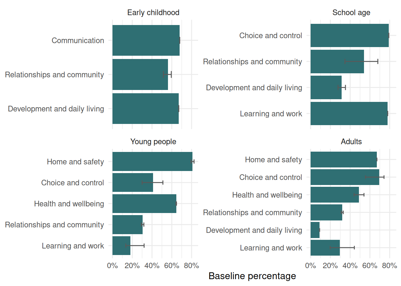
```{r}
#| label: baseline-theme-summary
#| fig-cap: "Median national baseline outcome level by participant cohort and outcome theme."
baseline_theme_summary <- participant_baseline |>
  group_by(cohort_label, outcome_theme) |>
  summarise(
    outcomes = n_distinct(indicator_description),
    median_level = safe_median(percentage),
    p25 = quantile(percentage, 0.25, na.rm = TRUE),
    p75 = quantile(percentage, 0.75, na.rm = TRUE),
    .groups = "drop"
  ) |>
  filter(is.finite(median_level))

baseline_theme_summary |>
  ggplot(aes(fct_reorder(outcome_theme, median_level), median_level)) +
  geom_col(fill = "#2f6f73") +
  geom_errorbar(aes(ymin = p25, ymax = p75), width = 0.2, colour = "grey35") +
  coord_flip() +
  facet_wrap(~ cohort_label, scales = "free_y") +
  scale_y_continuous(labels = percent) +
  labs(x = NULL, y = "Baseline percentage")
```
```{r}
#| label: baseline-level-table
participant_baseline |>
  arrange(cohort_label, outcome_theme, indicator_number) |>
  transmute(
    Cohort = as.character(cohort_label),
    Theme = outcome_theme,
    Outcome = indicator_description,
    Direction = direction,
    Level = percent(percentage, accuracy = 1)
  ) |>
  kable()
```
At baseline, the adult indicators show some obvious gaps as well as strengths. For example, many adults report choice over daily decisions and supports, but paid work and volunteering are much lower-level outcomes. For children, the outcome set is different: it is more about development, communication, friendships, community inclusion and school.
## Change After Reassessment
The cleanest first longitudinal comparison is baseline to reassessment 1 among national participant rows with one plan reassessment. This keeps the comparison simple and avoids mixing people with very different reassessment histories.
```{r}
#| label: reassessment-one-data
participant_reassessment1 <- participant_longitudinal |>
  filter(number_of_plan_reassessments == 1) |>
  transmute(
    cohort_label,
    outcome_theme,
    indicator_number,
    indicator_description,
    direction,
    baseline = percentage_baseline,
    reassessment_1 = percentage_reassessment_1,
    raw_change = reassessment_1 - baseline,
    direction_adjusted_change = direction_adjust_change(raw_change, direction)
  )

comparable_reassessment1 <- participant_reassessment1 |>
  filter(is.finite(baseline), is.finite(reassessment_1), is.finite(direction_adjusted_change))
```
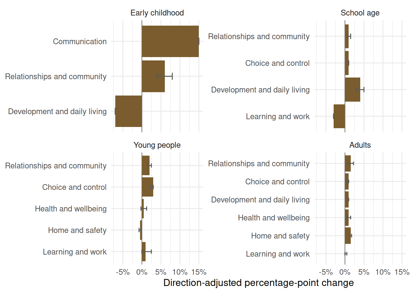
```{r}
#| label: reassessment-one-summary
#| fig-cap: "Median direction-adjusted change from baseline to reassessment 1."
reassessment1_summary <- comparable_reassessment1 |>
  group_by(cohort_label, outcome_theme) |>
  summarise(
    outcomes = n_distinct(indicator_description),
    median_change = safe_median(direction_adjusted_change),
    p25 = quantile(direction_adjusted_change, 0.25, na.rm = TRUE),
    p75 = quantile(direction_adjusted_change, 0.75, na.rm = TRUE),
    .groups = "drop"
  ) |>
  filter(is.finite(median_change))

reassessment1_summary |>
  ggplot(aes(fct_reorder(outcome_theme, median_change), median_change)) +
  geom_hline(yintercept = 0, colour = "grey60") +
  geom_col(fill = "#7a5c2e") +
  geom_errorbar(aes(ymin = p25, ymax = p75), width = 0.2, colour = "grey35") +
  coord_flip() +
  facet_wrap(~ cohort_label, scales = "free_y") +
  scale_y_continuous(labels = percent) +
  labs(x = NULL, y = "Direction-adjusted percentage-point change")
```
Most of the comparable indicators move in a favourable direction after the first reassessment, but the size varies. The table below keeps the raw baseline and reassessment percentages visible, then adds a direction-adjusted change only where the direction is clear.
```{r}
#| label: reassessment-one-table
comparable_reassessment1 |>
  mutate(abs_change = abs(direction_adjusted_change)) |>
  arrange(desc(abs_change)) |>
  slice_head(n = 25) |>
  transmute(
    Cohort = as.character(cohort_label),
    Theme = outcome_theme,
    Outcome = indicator_description,
    Direction = direction,
    Baseline = percent(baseline, accuracy = 1),
    `Reassessment 1` = percent(reassessment_1, accuracy = 1),
    `Raw change` = percent(raw_change, accuracy = 0.1),
    `Adjusted change` = percent(direction_adjusted_change, accuracy = 0.1)
  ) |>
  kable()
```
Some longitudinal items ask directly whether the NDIS helped or improved something. These do not have a meaningful baseline percentage, so they are better read as reassessment-level responses rather than baseline-to-reassessment changes.
```{r}
#| label: direct-improvement-items
direct_improvement_items <- participant_reassessment1 |>
  filter(is.na(baseline), is.finite(reassessment_1), direction == "Reported improvement") |>
  arrange(cohort_label, outcome_theme, indicator_number)

direct_improvement_items |>
  transmute(
    Cohort = as.character(cohort_label),
    Theme = outcome_theme,
    Outcome = indicator_description,
    `Reported improvement at reassessment 1` = percent(reassessment_1, accuracy = 1)
  ) |>
  kable()
```
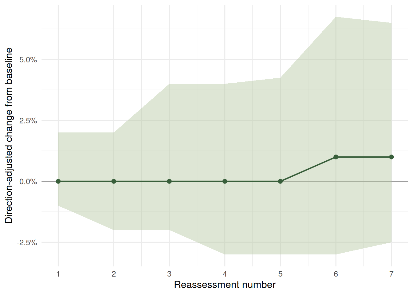
## Later Reassessments
The longitudinal file also includes reassessment 2 and later columns. Those are useful as a rough trend, but they should be read carefully: later reassessment rows are not a clean participant-level panel in this public extract, and the mix of participants changes as reassessment history gets longer.
```{r}
#| label: later-reassessment-trend
#| fig-cap: "Median direction-adjusted change by reassessment number."
reassessment_cols <- names(participant_longitudinal) |>
  keep(\(nm) str_detect(nm, "^percentage_reassessment_"))

participant_trend <- participant_longitudinal |>
  filter(
    is.finite(percentage_baseline),
    direction %in% c("Higher is better", "Lower is better")
  ) |>
  pivot_longer(
    all_of(reassessment_cols),
    names_to = "reassessment",
    values_to = "reassessment_value"
  ) |>
  mutate(
    reassessment_number = as.integer(str_extract(reassessment, "[0-9]+")),
    raw_change = reassessment_value - percentage_baseline,
    direction_adjusted_change = direction_adjust_change(raw_change, direction)
  ) |>
  filter(
    reassessment_number <= number_of_plan_reassessments,
    reassessment_number <= 7,
    is.finite(direction_adjusted_change)
  )

trend_summary <- participant_trend |>
  group_by(reassessment_number) |>
  summarise(
    rows = n(),
    outcome_cohort_pairs = n_distinct(str_c(cohort_label, indicator_number, sep = "::")),
    median_change = safe_median(direction_adjusted_change),
    p25 = quantile(direction_adjusted_change, 0.25, na.rm = TRUE),
    p75 = quantile(direction_adjusted_change, 0.75, na.rm = TRUE),
    .groups = "drop"
  ) |>
  filter(rows >= 20)

if (nrow(trend_summary) > 0) {
  trend_summary |>
    ggplot(aes(reassessment_number, median_change)) +
    geom_hline(yintercept = 0, colour = "grey60") +
    geom_ribbon(aes(ymin = p25, ymax = p75), fill = "#b7c7a3", alpha = 0.45) +
    geom_line(colour = "#395f3b", linewidth = 0.8) +
    geom_point(colour = "#395f3b", size = 2) +
    scale_x_continuous(breaks = trend_summary$reassessment_number) +
    scale_y_continuous(labels = percent) +
    labs(x = "Reassessment number", y = "Direction-adjusted change from baseline")
} else {
  tibble(note = "There are not enough later reassessment rows to draw a stable trend.") |>
    kable()
}
```
```{r}
#| label: later-reassessment-table
trend_summary |>
  transmute(
    Reassessment = reassessment_number,
    Rows = comma(rows),
    `Outcome/cohort pairs` = outcome_cohort_pairs,
    `Median adjusted change` = percent(median_change, accuracy = 0.1),
    `25th percentile` = percent(p25, accuracy = 0.1),
    `75th percentile` = percent(p75, accuracy = 0.1)
  ) |>
  kable()
```
The later-reassessment pattern is best read as directional context, not as a precise individual trajectory. Still, it helps separate the first question from the bigger spend question: the public data does show reported outcome movement after entry, even before we try to link those changes to budgets, service markets or regional access.
## Family And Carer Note
Family and carer outcomes are part of the public outcomes files, but they answer a different question. They are about the circumstances of the family or carer around the participant, not the participant's own outcome level. For this reason, they sit beside the participant story rather than inside it.
```{r}
#| label: family-carer-summary
family_reassessment1 <- family_longitudinal |>
  filter(number_of_plan_reassessments == 1) |>
  transmute(
    cohort_label,
    outcome_theme,
    indicator_description,
    direction,
    baseline = percentage_baseline,
    reassessment_1 = percentage_reassessment_1,
    raw_change = reassessment_1 - baseline,
    direction_adjusted_change = direction_adjust_change(raw_change, direction)
  )

family_summary <- family_reassessment1 |>
  group_by(cohort_label) |>
  summarise(
    comparable_outcomes = sum(is.finite(direction_adjusted_change)),
    median_adjusted_change = safe_median(direction_adjusted_change),
    direct_improvement_items = sum(is.na(baseline) & is.finite(reassessment_1)),
    median_direct_improvement = safe_median(reassessment_1[is.na(baseline) & is.finite(reassessment_1)]),
    .groups = "drop"
  )

family_summary |>
  transmute(
    Cohort = as.character(cohort_label),
    `Comparable outcomes` = comparable_outcomes,
    `Median adjusted change` = format_optional_percent(median_adjusted_change, accuracy = 0.1),
    `Direct improvement items` = direct_improvement_items,
    `Median direct improvement response` = format_optional_percent(median_direct_improvement, accuracy = 1)
  ) |>
  kable()
```
The family and carer rows are useful, especially for questions about informal care, work, confidence, health and service access. They should not be blended with participant rows when the main question is whether participant outcomes themselves changed.
## Caveats
- These are aggregate public survey rows, not participant-level records.
- The reassessment comparisons are descriptive. They do not prove causation.
- Later reassessment rows may reflect a different participant mix from earlier reassessment rows.
- Direction-adjusting outcomes helps readability, but it does not make all indicators equally important.
- Some items ask whether the NDIS helped or improved something. Those are reassessment responses, not true baseline-to-change measures.
- Spend, provider access and regional service-market questions are deliberately left out of this simplified version.